如何在Python中进行指数和对数曲线拟合？我只找到了多项式拟合。

Question

我有一组数据，想要比较哪条线最能够描述它（不同阶数的多项式、指数或对数函数）。

我使用Python和Numpy，对于多项式拟合，有一个名为polyfit()的函数。但是我没有找到指数和对数函数的拟合函数。

是否有这样的函数？否则该如何解决？

- Tomas Novotny

Answer 1

对于拟合 y = A + B log x，只需将y与（log x）进行拟合。

>>> x = numpy.array([1, 7, 20, 50, 79])
>>> y = numpy.array([10, 19, 30, 35, 51])
>>> numpy.polyfit(numpy.log(x), y, 1)
array([ 8.46295607,  6.61867463])
# y ≈ 8.46 log(x) + 6.62

---

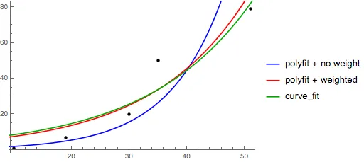
对于拟合y = Ae^Bx，取两边的对数得到log y = log A + Bx。因此，拟合(log y)与x。

请注意，将(log y)视为线性拟合会强调y的小值，导致大y的偏差很大。这是因为polyfit（线性回归）通过最小化∑_i (ΔY)² = ∑_i (Y_i − Ŷ_i)²来工作。当Y_i = log y_i时，残差ΔY_i = Δ(log y_i) ≈ Δy_i / |y_i|。因此，即使polyfit对大y做出了非常糟糕的决策，"除以|y|"因子也会进行补偿，使polyfit更倾向于小值。

这可以通过为每个条目分配与y成比例的“权重”来缓解。 polyfit 支持通过w关键字参数进行加权最小二乘法。

>>> x = numpy.array([10, 19, 30, 35, 51])
>>> y = numpy.array([1, 7, 20, 50, 79])
>>> numpy.polyfit(x, numpy.log(y), 1)
array([ 0.10502711, -0.40116352])
#    y ≈ exp(-0.401) * exp(0.105 * x) = 0.670 * exp(0.105 * x)
# (^ biased towards small values)
>>> numpy.polyfit(x, numpy.log(y), 1, w=numpy.sqrt(y))
array([ 0.06009446,  1.41648096])
#    y ≈ exp(1.42) * exp(0.0601 * x) = 4.12 * exp(0.0601 * x)
# (^ not so biased)

请注意，Excel、LibreOffice和大多数科学计算器通常使用带偏差的未加权公式进行指数回归/趋势线计算。如果您希望您的结果与这些平台兼容，请不要包括权重，即使它能够提供更好的结果。

---

现在，如果您可以使用scipy，您可以使用scipy.optimize.curve_fit来拟合任何模型而无需进行转换。

对于y = A + B log x，结果与转换方法相同：

>>> x = numpy.array([1, 7, 20, 50, 79])
>>> y = numpy.array([10, 19, 30, 35, 51])
>>> scipy.optimize.curve_fit(lambda t,a,b: a+b*numpy.log(t),  x,  y)
(array([ 6.61867467,  8.46295606]), 
 array([[ 28.15948002,  -7.89609542],
        [ -7.89609542,   2.9857172 ]]))
# y ≈ 6.62 + 8.46 log(x)

然而，对于y=Ae^Bx，我们可以得到更好的拟合，因为它直接计算Δ(logy)。但是我们需要提供一个初始化猜测，以便curve_fit可以达到所需的局部最小值。

>>> x = numpy.array([10, 19, 30, 35, 51])
>>> y = numpy.array([1, 7, 20, 50, 79])
>>> scipy.optimize.curve_fit(lambda t,a,b: a*numpy.exp(b*t),  x,  y)
(array([  5.60728326e-21,   9.99993501e-01]),
 array([[  4.14809412e-27,  -1.45078961e-08],
        [ -1.45078961e-08,   5.07411462e+10]]))
# oops, definitely wrong.
>>> scipy.optimize.curve_fit(lambda t,a,b: a*numpy.exp(b*t),  x,  y,  p0=(4, 0.1))
(array([ 4.88003249,  0.05531256]),
 array([[  1.01261314e+01,  -4.31940132e-02],
        [ -4.31940132e-02,   1.91188656e-04]]))
# y ≈ 4.88 exp(0.0553 x). much better.

- kennytm

---

@Tomas：没错。改变对数的底只是将一个常数乘以log x或log y，这不会影响r^2。 - kennytm

这将更加强调小y处的价值。因此，最好通过对y_i进行加权来对卡方值的贡献进行加权。 - Rupert Nash

传统曲线拟合中，这种解决方案是错误的。它不会在线性空间中最小化残差平方和，而是在对数空间中。如前所述，这实际上改变了点的加权方式--当y较小时的观测值将被人为赋予更大的权重。最好定义函数（线性函数，而不是对数变换）并使用曲线拟合器或最小化器。 - santon

@santon 解决了指数回归中的偏差问题。 - kennytm

谢谢你添加权重！许多/大多数人不知道，如果你只是取log（data）并通过它运行一条线（比如Excel），结果可能非常糟糕，甚至滑稽可笑。就像我之前多年一直在做的那样。当我的贝叶斯老师向我展示这个时，我感到很惊讶，"但他们不是会在物理学中教授[错误]的方法吗？" - "是的，我们称之为 '婴儿物理学'，这是一种简化。这才是正确的方法。" - DeusXMachina

Answer 2

你也可以使用来自scipy.optimize的curve_fit将一组数据拟合到任何你喜欢的函数中。例如，如果您想要拟合一个指数函数（请参见文档）：

import numpy as np
import matplotlib.pyplot as plt
from scipy.optimize import curve_fit

def func(x, a, b, c):
    return a * np.exp(-b * x) + c

x = np.linspace(0,4,50)
y = func(x, 2.5, 1.3, 0.5)
yn = y + 0.2*np.random.normal(size=len(x))

popt, pcov = curve_fit(func, x, yn)

然后如果您想绘图，可以执行以下操作：

plt.figure()
plt.plot(x, yn, 'ko', label="Original Noised Data")
plt.plot(x, func(x, *popt), 'r-', label="Fitted Curve")
plt.legend()
plt.show()

（注意：当你绘制时，在popt前的*会将项展开为func所期望的a, b和c。）

- IanVS

---

好的。有没有一种方法可以检查我们得到了多好的适合度？R平方值？是否有不同的优化算法参数可尝试以获得更好（或更快）的解决方案？ - user391339

为了拟合优度，您可以将拟合的优化参数传递给scipy optimize函数chisquare；它返回2个值，其中第二个是p值。 - user7345804

有没有关于如何选择参数 a、b 和 c 的想法？ - Gilfoyle

@Samuel，或许有点晚了，但是在 @Leandro 的回答中有这样的代码：popt[0] = a , popt[1] = b, popt[2] = c。 - willcrack

Answer 3

我在处理这个问题时遇到了一些麻烦，所以让我非常明确，以便像我这样的新手能够理解。

假设我们有一个数据文件或类似的东西。

# -*- coding: utf-8 -*-

import matplotlib.pyplot as plt
from scipy.optimize import curve_fit
import numpy as np
import sympy as sym

"""
Generate some data, let's imagine that you already have this. 
"""
x = np.linspace(0, 3, 50)
y = np.exp(x)

"""
Plot your data
"""
plt.plot(x, y, 'ro',label="Original Data")

"""
brutal force to avoid errors
"""    
x = np.array(x, dtype=float) #transform your data in a numpy array of floats 
y = np.array(y, dtype=float) #so the curve_fit can work

"""
create a function to fit with your data. a, b, c and d are the coefficients
that curve_fit will calculate for you. 
In this part you need to guess and/or use mathematical knowledge to find
a function that resembles your data
"""
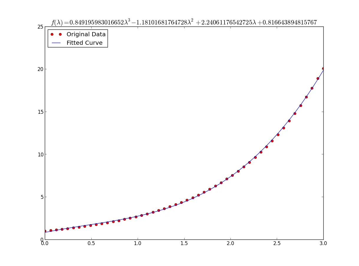
def func(x, a, b, c, d):
    return a*x**3 + b*x**2 +c*x + d

"""
make the curve_fit
"""
popt, pcov = curve_fit(func, x, y)

"""
The result is:
popt[0] = a , popt[1] = b, popt[2] = c and popt[3] = d of the function,
so f(x) = popt[0]*x**3 + popt[1]*x**2 + popt[2]*x + popt[3].
"""
print "a = %s , b = %s, c = %s, d = %s" % (popt[0], popt[1], popt[2], popt[3])

"""
Use sympy to generate the latex sintax of the function
"""
xs = sym.Symbol('\lambda')    
tex = sym.latex(func(xs,*popt)).replace('$', '')
plt.title(r'$f(\lambda)= %s$' %(tex),fontsize=16)

"""
Print the coefficients and plot the funcion.
"""

plt.plot(x, func(x, *popt), label="Fitted Curve") #same as line above \/
#plt.plot(x, popt[0]*x**3 + popt[1]*x**2 + popt[2]*x + popt[3], label="Fitted Curve") 

plt.legend(loc='upper left')
plt.show()

结果为：a = 0.849195983017，b = -1.18101681765，c = 2.24061176543，d = 0.816643894816。

- Leandro

---

y = [np.exp(i) for i in x] 的速度非常慢；Numpy 库的其中一个用途就是让你可以写成 y=np.exp(x)。此外，使用这个替换后，你可以摆脱冗长的循环代码块。在 ipython 中，有 %timeit 魔法命令可以用来测试运行时间：In [27]: %timeit ylist=[exp(i) for i in x] 10000 loops, best of 3: 172 us per loop In [28]: %timeit yarr=exp(x) 100000 loops, best of 3: 2.85 us per loop - esmit

谢谢esmit，你是对的，但是当我处理来自csv、xls或其他格式的数据时，我仍然需要使用暴力部分。我认为只有在某人试图从实验或模拟数据中拟合函数时，才有意义使用它，在我的经验中，这些数据总是以奇怪的格式出现。 - Leandro

x = np.array(x, dtype=float) 可以让你摆脱缓慢的列表推导式。 - Ajasja

Answer 4

这里有一个使用来自scikit learn工具的简单数据的线性化选项。

import numpy as np

import matplotlib.pyplot as plt

from sklearn.linear_model import LinearRegression
from sklearn.preprocessing import FunctionTransformer


np.random.seed(123)

# General Functions
def func_exp(x, a, b, c):
    """Return values from a general exponential function."""
    return a * np.exp(b * x) + c


def func_log(x, a, b, c):
    """Return values from a general log function."""
    return a * np.log(b * x) + c


# Helper
def generate_data(func, *args, jitter=0):
    """Return a tuple of arrays with random data along a general function."""
    xs = np.linspace(1, 5, 50)
    ys = func(xs, *args)
    noise = jitter * np.random.normal(size=len(xs)) + jitter
    xs = xs.reshape(-1, 1)                                  # xs[:, np.newaxis]
    ys = (ys + noise).reshape(-1, 1)
    return xs, ys

transformer = FunctionTransformer(np.log, validate=True)

代码

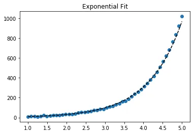
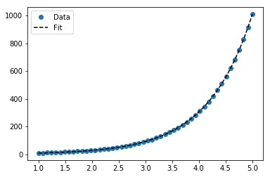
拟合指数数据

# Data
x_samp, y_samp = generate_data(func_exp, 2.5, 1.2, 0.7, jitter=3)
y_trans = transformer.fit_transform(y_samp)             # 1

# Regression
regressor = LinearRegression()
results = regressor.fit(x_samp, y_trans)                # 2
model = results.predict
y_fit = model(x_samp)

# Visualization
plt.scatter(x_samp, y_samp)
plt.plot(x_samp, np.exp(y_fit), "k--", label="Fit")     # 3
plt.title("Exponential Fit")

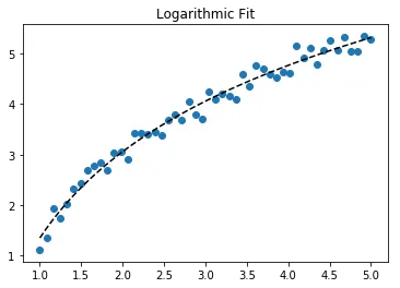
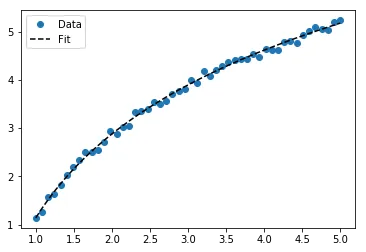
适配日志数据

# Data
x_samp, y_samp = generate_data(func_log, 2.5, 1.2, 0.7, jitter=0.15)
x_trans = transformer.fit_transform(x_samp)             # 1

# Regression
regressor = LinearRegression()
results = regressor.fit(x_trans, y_samp)                # 2
model = results.predict
y_fit = model(x_trans)

# Visualization
plt.scatter(x_samp, y_samp)
plt.plot(x_samp, y_fit, "k--", label="Fit")             # 3
plt.title("Logarithmic Fit")

---

详情

通用步骤

1. 对数据值（x、y 或两者）应用对数操作
2. 将数据回归到线性模型中
3. 通过“反转”任何对数操作（使用 np.exp()）绘制图表并拟合原始数据

假设我们的数据遵循指数趋势，则通用方程式⁺可能为：

我们可以通过取对数来线性化后一个方程式（例如 y = intercept + slope * x）：

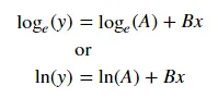
给定线性化方程式⁺⁺和回归参数，我们可以计算：

• 通过截距计算 A（ln(A)）
• 通过斜率计算 B（B）

线性化技术摘要

Relationship |  Example   |     General Eqn.     |  Altered Var.  |        Linearized Eqn.  
-------------|------------|----------------------|----------------|------------------------------------------
Linear       | x          | y =     B * x    + C | -              |        y =   C    + B * x
Logarithmic  | log(x)     | y = A * log(B*x) + C | log(x)         |        y =   C    + A * (log(B) + log(x))
Exponential  | 2**x, e**x | y = A * exp(B*x) + C | log(y)         | log(y-C) = log(A) + B * x
Power        | x**2       | y =     B * x**N + C | log(x), log(y) | log(y-C) = log(B) + N * log(x)

_{⁺注意：在线性化指数函数时，当噪声较小且C=0时效果最好。请谨慎使用。}

_{⁺⁺注意：尽管改变x数据有助于线性化指数数据，但改变y数据有助于线性化对数数据。}

- pylang

Answer 5

好的，我想你总是可以使用：

np.log   -->  natural log
np.log10 -->  base 10
np.log2  -->  base 2

稍微修改IanVS答案的方法：

原答案在此:

import numpy as np
import matplotlib.pyplot as plt
from scipy.optimize import curve_fit

def func(x, a, b, c):
  #return a * np.exp(-b * x) + c
  return a * np.log(b * x) + c

x = np.linspace(1,5,50)   # changed boundary conditions to avoid division by 0
y = func(x, 2.5, 1.3, 0.5)
yn = y + 0.2*np.random.normal(size=len(x))

popt, pcov = curve_fit(func, x, yn)

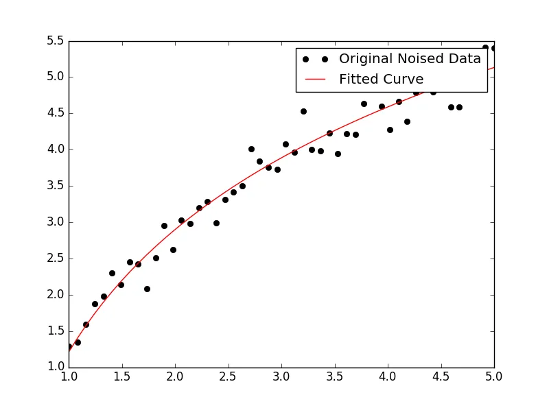
plt.figure()
plt.plot(x, yn, 'ko', label="Original Noised Data")
plt.plot(x, func(x, *popt), 'r-', label="Fitted Curve")
plt.legend()
plt.show()

这导致了以下的图形：

- murphy1310

---

拟合是否有饱和值？如果有，如何访问它？ - Ben

然而，需要注意的是，图例呈现出一张没有表情的脸。 - reynoldsnlp

Answer 6

我们在解决这两个问题时展示了 lmfit 的特点。

给定

import lmfit

import numpy as np

import matplotlib.pyplot as plt


%matplotlib inline
np.random.seed(123)

# General Functions
def func_log(x, a, b, c):
    """Return values from a general log function."""
    return a * np.log(b * x) + c


# Data
x_samp = np.linspace(1, 5, 50)
_noise = np.random.normal(size=len(x_samp), scale=0.06)
y_samp = 2.5 * np.exp(1.2 * x_samp) + 0.7 + _noise
y_samp2 = 2.5 * np.log(1.2 * x_samp) + 0.7 + _noise

代码

方法1 - lmfit模型

拟合指数数据

regressor = lmfit.models.ExponentialModel()                # 1    
initial_guess = dict(amplitude=1, decay=-1)                # 2
results = regressor.fit(y_samp, x=x_samp, **initial_guess)
y_fit = results.best_fit    

plt.plot(x_samp, y_samp, "o", label="Data")
plt.plot(x_samp, y_fit, "k--", label="Fit")
plt.legend()

方法2 - 自定义模型

适配日志数据

regressor = lmfit.Model(func_log)                          # 1
initial_guess = dict(a=1, b=.1, c=.1)                      # 2
results = regressor.fit(y_samp2, x=x_samp, **initial_guess)
y_fit = results.best_fit

plt.plot(x_samp, y_samp2, "o", label="Data")
plt.plot(x_samp, y_fit, "k--", label="Fit")
plt.legend()

---

细节：

1. 选择回归类别
2. 提供命名的、初始的猜测值，以尊重函数的定义域

您可以从回归器对象中确定推断出的参数。例如：

regressor.param_names
# ['decay', 'amplitude']

使用 ModelResult.eval() 方法来 进行预测。

model = results.eval
y_pred = model(x=np.array([1.5]))

注意：`ExponentialModel()` 遵循一个衰减函数，它接受两个参数，其中一个是负数。

请参阅 ExponentialGaussianModel()，它接受更多的参数。

通过> pip install lmfit 安装该库。

- pylang

Answer 7

Wolfram提供了指数拟合的封闭形式解法。他们还提供了类似的解决方案来适应对数和幂律。

我发现这比scipy的curve_fit更有效，特别是当你没有“接近零”的数据时。以下是一个例子：

import numpy as np
import matplotlib.pyplot as plt

# Fit the function y = A * exp(B * x) to the data
# returns (A, B)
# From: https://mathworld.wolfram.com/LeastSquaresFittingExponential.html
def fit_exp(xs, ys):
    S_x2_y = 0.0
    S_y_lny = 0.0
    S_x_y = 0.0
    S_x_y_lny = 0.0
    S_y = 0.0
    for (x,y) in zip(xs, ys):
        S_x2_y += x * x * y
        S_y_lny += y * np.log(y)
        S_x_y += x * y
        S_x_y_lny += x * y * np.log(y)
        S_y += y
    #end
    a = (S_x2_y * S_y_lny - S_x_y * S_x_y_lny) / (S_y * S_x2_y - S_x_y * S_x_y)
    b = (S_y * S_x_y_lny - S_x_y * S_y_lny) / (S_y * S_x2_y - S_x_y * S_x_y)
    return (np.exp(a), b)


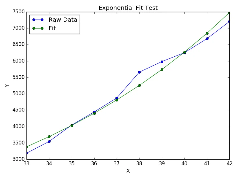
xs = [33, 34, 35, 36, 37, 38, 39, 40, 41, 42]
ys = [3187, 3545, 4045, 4447, 4872, 5660, 5983, 6254, 6681, 7206]

(A, B) = fit_exp(xs, ys)

plt.figure()
plt.plot(xs, ys, 'o-', label='Raw Data')
plt.plot(xs, [A * np.exp(B *x) for x in xs], 'o-', label='Fit')

plt.title('Exponential Fit Test')
plt.xlabel('X')
plt.ylabel('Y')
plt.legend(loc='best')
plt.tight_layout()
plt.show()

- Ben