使用plm和pglm绘制面板模型预测

Question

我使用plm创建了一个线性面板模型和使用pglm包的泊松广义面板模型，共创建了两个回归模型。

library(plm); library(pglm)
data(Unions)  # from pglm-package
punions <- pdata.frame(Unions, c("id", "year"))

fit1 <- plm(wage ~ exper + rural + married, data=punions, model="random")
fit2 <- pglm(wage ~ exper + rural + married, data=punions, model="random", family="poisson")

我现在想通过绘制一组散点图来以图形方式比较这两个拟合值。最好使用 ggplot2 实现：

library(ggplot2)
ggplot(punions, aes(x=exper, y=wage)) +
    geom_point() +
    facet_wrap(rural ~ married)

我考虑使用ggplot2的stat_smooth()，但是（也许并不奇怪）它似乎不能识别我的数据的面板格式。使用predict手动提取预测值也似乎对pglm模型无效。

如何在此图中叠加我的两个面板模型的预测值？

- ageil

---

这个文档页面中间的示例可能对你有用。 - asachet

你的随机效应是什么？个体吗？ - alexwhitworth

Answer 1

与 @mtoto 类似，我也不熟悉 library(plm) 或 library(pglm)。但是，plm 的预测方法可用，只是没有被导出。 编辑：对于由 plm::plm() 生成的模型，自从 plm CRAN 版本 2.6-2 发布以来，有一个可用的 predict 方法。pglm 没有预测方法。

R> methods(class= "plm")
[1] ercomp          fixef           has.intercept   model.matrix    pFtest          plmtest         plot            pmodel.response
 [9] pooltest        predict         residuals       summary         vcovBK          vcovHC          vcovSCC        
R> methods(class= "pglm")
no methods found

值得注意的是，我不明白为什么你在工资数据中使用泊松模型。显然这不是一个泊松分布，因为它采用了非整数值（如下所示）。如果您愿意，可以尝试负二项式，但我不确定是否可以使用随机效应。但是您可以使用MASS::glm.nb。

> quantile(Unions$wage, seq(0,1,.1))
         0%         10%         20%         30%         40%         50%         60%         70%         80%         90%        100% 
 0.02790139  2.87570334  3.54965422  4.14864865  4.71605855  5.31824370  6.01422463  6.87414349  7.88514525  9.59904809 57.50431282

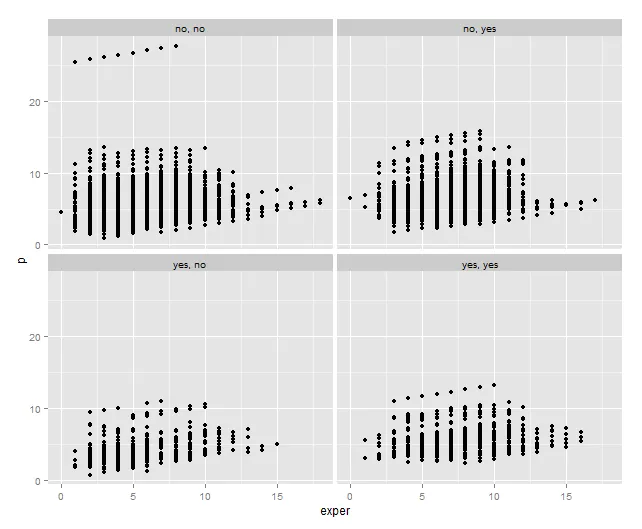
解决方案1：使用plm

punions$p <- predict(fit1, punions)

ggplot(punions, aes(x=exper, y=p)) +
  geom_point() +
  facet_wrap(rural ~ married) 

方案2 - lme4

或者，您可以使用lme4软件包获取类似的拟合结果，该软件包已定义了预测方法：

library(lme4)
Unions$id <- factor(Unions$id)
fit3 <- lmer(wage ~ exper + rural + married + (1|id), data= Unions)
# not run:
fit4 <- glmer(wage ~ exper + rural + married + (1|id), data= Unions, family= poisson(link= "log"))

R> fit1$coefficients
(Intercept)       exper    ruralyes  marriedyes 
  3.7467469   0.3088949  -0.2442846   0.4781113 
R>  fixef(fit3)
(Intercept)       exper    ruralyes  marriedyes 
  3.7150302   0.3134898  -0.1950361   0.4592975 

我还没有运行泊松模型，因为它的规范明显是错误的。你可以进行某种变量转换来处理，或者使用负二项式。无论如何，让我们完成这个例子:

# this has RE for individuals, so you do see dispersion based on the RE
Unions$p <- predict(fit3, Unions)
ggplot(Unions, aes(x=exper, y=p)) +
    geom_point() +
    facet_wrap(rural ~ married)

- alexwhitworth

---

对于由 plm::plm() 生成的模型，自 plm 版本2.6-2 起提供了 predict 方法。 - Helix123

Answer 2

我不熟悉pglm包，但似乎没有类似于predict()的函数可以从数据帧生成未来值的向量。

在所有其他情况下（应该都是这样），您可以轻松地在ggplot中绘制它，甚至使用facet wrap。您只需将预测添加到数据框作为新列：

punions$pred1 <- predict(fit1,punions,class="lm")

然后将其作为额外的 geom_line() 添加：

    ggplot() + geom_point(data=punions, aes(x=exper, y=wage)) +
    geom_line(data=punions,aes(x=exper, y= pred1), color = "red") +
    facet_wrap(rural ~ married)

- mtoto