我使用的是Debian squeeze上的R 2.15.3(2013-03-01),ggplot2_0.9.3.1,lattice_0.20-13,gtable_0.1.2,gridExtra_0.9.1。
请考虑
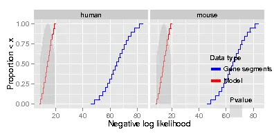
minimal.R 生成的图表。这与我的实际图表类似。########################
minimal.R
########################
get_stat <- function()
{
n = 20
q1 = qnorm(seq(3, 17)/20, 14, 5)
q2 = qnorm(seq(1, 19)/20, 65, 10)
Stat = data.frame(value = c(q1, q2),
pvalue = c(dnorm(q1, 14, 5)/max(dnorm(q1, 14, 5)), d = dnorm(q2, 65, 10)/max(dnorm(q2, 65, 10))),
variable = c(rep('true', length(q1)), rep('data', length(q2))))
return(Stat)
}
stat_all<- function()
{
library(ggplot2)
library(gridExtra)
stathuman = get_stat()
stathuman$dataset = "human"
statmouse = get_stat()
statmouse$dataset = "mouse"
stat = merge(stathuman, statmouse, all=TRUE)
return(stat)
}
simplot <- function()
{
Stat = stat_all()
Pvalue = subset(Stat, variable=="true")
pdf(file = "CDF.pdf", width = 5.5, height = 2.7)
stat = ggplot() + stat_ecdf(data=Stat, n=1000, aes(x=value, colour = variable)) +
theme(legend.key = element_blank(), legend.background = element_blank(), legend.position=c(.9, .25), legend.title = element_text(face = "bold")) +
scale_x_continuous("Negative log likelihood") +
scale_y_continuous("Proportion $<$ x") +
facet_grid(~ dataset, scales='free') +
scale_colour_manual(values = c("blue", "red"), name="Data type",
labels=c("Gene segments", "Model"), guide=guide_legend(override.aes = list(size = 2))) +
geom_area(data=Pvalue, aes(x=value, y=pvalue, fill=variable), position="identity", alpha=0.5) +
scale_fill_manual(values = c("gray"), name="Pvalue", labels=c(""))
print(stat)
dev.off()
}
simplot()
这导致产生以下图表。可以看出,
数据类型和P值图例的位置不太合适。我将该代码修改为 minimal2.R。
使用应该将图例放在顶部的第一个版本时,代码运行没有错误,但没有显示图例。
编辑:显示两个框,一个在另一个上面。上面那个是空白的。如果我不在grid.arrange()中设置高度,如@baptiste所建议的那样,则图例和图表都会放在底部框中。
如果我设置了如下的高度,则看不到图例。
编辑2:似乎多余的空白框由grid.newpage引起,我从早期问题中复制了这个框。我不确定它为什么会在那里。如果我不使用那一行,则只会得到一个框/页面。
使用第二个版本时,我遇到了这个错误。
Error in UseMethod("grid.draw") :
  no applicable method for 'grid.draw' applied to an object of class "c('gg', 'ggplot')"
Calls: simplot -> grid.draw
编辑:如果我像@baptiste建议的那样使用print(plotNew),则会出现以下错误
Error in if (empty(data)) { : missing value where TRUE/FALSE needed
Calls: simplot ... facet_map_layout -> facet_map_layout.grid -> locate_grid.
我试图弄清楚这里发生了什么事情,但是我没有找到太多相关信息。
注:
I'm not sure why I'm getting the staircase effect for the empirical CDF. I'm sure there is an obvious explanation. Please enlighten me if you know.
I'm willing to consider alternatives to this code and even ggplot2 for producing this graph, if anyone can suggest alternatives, e.g. matplotlib, which I have never seriously experimented with.
Adding
print(ggplot_gtable(ggplot_build(stat2)))to
minimal2.Rgives meTableGrob (7 x 7) "layout": 12 grobs z cells name grob 1 0 (1-7,1-7) background rect[plot.background.rect.186] 2 1 (3-3,4-4) strip-top absoluteGrob[strip.absoluteGrob.135] 3 2 (3-3,6-6) strip-top absoluteGrob[strip.absoluteGrob.141] 4 5 (4-4,3-3) axis-l absoluteGrob[GRID.absoluteGrob.129] 5 3 (4-4,4-4) panel gTree[GRID.gTree.155] 6 4 (4-4,6-6) panel gTree[GRID.gTree.169] 7 6 (5-5,4-4) axis-b absoluteGrob[GRID.absoluteGrob.117] 8 7 (5-5,6-6) axis-b absoluteGrob[GRID.absoluteGrob.123] 9 8 (6-6,4-6) xlab text[axis.title.x.text.171] 10 9 (4-4,2-2) ylab text[axis.title.y.text.173] 11 10 (4-4,4-6) guide-box gtable[guide-box] 12 11 (2-2,4-6) title text[plot.title.text.184]I don't understand this breakdown. Can anyone explain? Does
guide-boxcorrespond to the legend, and how does one know this?
这是我修改后的代码版本,minimal2.R。
########################
minimal2.R
########################

get_stat <- function()
  {
    n = 20
    q1 = qnorm(seq(3, 17)/20, 14, 5)
    q2 = qnorm(seq(1, 19)/20, 65, 10)
    Stat = data.frame(value = c(q1, q2),
      pvalue = c(dnorm(q1, 14, 5)/max(dnorm(q1, 14, 5)), d = dnorm(q2, 65, 10)/max(dnorm(q2, 65, 10))),
      variable = c(rep('true', length(q1)), rep('data', length(q2))))
    return(Stat)
  }

stat_all<- function()
{
  library(ggplot2)
  library(gridExtra)
  library(gtable)
  stathuman = get_stat()
  stathuman$dataset = "human"
  statmouse = get_stat()
  statmouse$dataset = "mouse"
  stat = merge(stathuman, statmouse, all=TRUE)
  return(stat)
}

simplot <- function()
  {
    Stat = stat_all()
    Pvalue = subset(Stat, variable=="true")
    pdf(file = "CDF.pdf", width = 5.5, height = 2.7)

    ## only include data type legend
    stat1 = ggplot() + stat_ecdf(data=Stat, n=1000, aes(x=value, colour = variable)) +
      theme(legend.key = element_blank(), legend.background = element_blank(), legend.position=c(.9, .25), legend.title = element_text(face = "bold")) +
        scale_x_continuous("Negative log likelihood") +
          scale_y_continuous("Proportion $<$ x") +
            facet_grid(~ dataset, scales='free') +
              scale_colour_manual(values = c("blue", "red"), name="Data type", labels=c("Gene segments", "Model"), guide=guide_legend(override.aes = list(size = 2))) +
                geom_area(data=Pvalue, aes(x=value, y=pvalue, fill=variable), position="identity", alpha=0.5) +
                  scale_fill_manual(values = c("gray"), name="Pvalue", labels=c(""), guide=FALSE)

    ## Extract data type legend
    dataleg <- gtable_filter(ggplot_gtable(ggplot_build(stat1)), "guide-box")

    ## only include pvalue legend
    stat2 = ggplot() + stat_ecdf(data=Stat, n=1000, aes(x=value, colour = variable)) +
      theme(legend.key = element_blank(), legend.background = element_blank(), legend.position=c(.9, .25), legend.title = element_text(face = "bold")) +
        scale_x_continuous("Negative log likelihood") +
          scale_y_continuous("Proportion $<$ x") +
            facet_grid(~ dataset, scales='free') +
              scale_colour_manual(values = c("blue", "red"), name="Data type", labels=c("Gene segments", "Model"), guide=FALSE) +
                geom_area(data=Pvalue, aes(x=value, y=pvalue, fill=variable), position="identity", alpha=0.5) +
                  scale_fill_manual(values = c("gray"), name="Pvalue", labels=c(""))

    ## Extract pvalue legend
    pvalleg <- gtable_filter(ggplot_gtable(ggplot_build(stat2)), "guide-box")

    ## no legends
    stat = ggplot() + stat_ecdf(data=Stat, n=1000, aes(x=value, colour = variable)) +
      theme(legend.key = element_blank(), legend.background = element_blank(), legend.position=c(.9, .25), legend.title = element_text(face = "bold")) +
        scale_x_continuous("Negative log likelihood") +
          scale_y_continuous("Proportion $<$ x") +
            facet_grid(~ dataset, scales='free') +
              scale_colour_manual(values = c("blue", "red"), name="Data type", labels=c("Gene segments", "Model"), guide=FALSE) +
                geom_area(data=Pvalue, aes(x=value, y=pvalue, fill=variable), position="identity", alpha=0.5) +
                  scale_fill_manual(values = c("gray"), name="Pvalue", labels=c(""), guide=FALSE)

    ## Add data type legend: version 1 (data type legend should be on top)
    ## plotNew <- arrangeGrob(dataleg, stat, heights = unit.c(dataleg$height, unit(1, "npc") - dataleg$height), ncol = 1)

    ## Add data type legend: version 2 (data type legend should be somewhere in the interior)
    ## plotNew <- stat + annotation_custom(grob = dataleg, xmin = 7, xmax = 10, ymin = 0, ymax = 4)

    grid.newpage()
    grid.draw(plotNew)
    dev.off()
  }

simplot()
grid.arrange()中设置高度(我还没有尝试过你的代码)。 - baptistegrid.draw替换为print(plotNew)会导致以下错误:if (empty(data)) { : missing value where TRUE/FALSE needed Calls: simplot ... facet_map_layout -> facet_map_layout.grid -> locate_grid。对于第一个版本,不设置高度有点奏效。它会产生两个相互重叠的框,但是顶部的框为空,底部的框包含图例和绘图。 - Faheem Mitha