如何在ggplot中独立定位两个图例

Question

标题已经很好地概括了问题。

我有两个图例，一个是有关大小的，一个是有关颜色的，并希望将一个放在顶部，另一个放在图表内部。

是否可行，如果可以，请问如何实现？

谢谢您的帮助。

- pssguy

---

我认为这是不可能的（图例的位置由主题控制，定义图例位置的部分只有一个值）。然而，我不确定是否能将其作为答案。 - Brian Diggs

猜测如果是这样的话，专家们现在应该已经在场了。 - pssguy

@pssguy，这可以通过一些调整来完成。为了对图例进行控制，您需要提取单独的图例，然后将它们排列在最初不包含图例的图中。 - Sandy Muspratt

Answer 1

可以通过从图表中提取单独的图例，然后将这些图例排列在相关的图表中来完成。此处的代码使用 gtable 包中的函数进行提取，然后使用 gridExtra 包中的函数进行排列。目标是拥有一个包含颜色图例和大小图例的图表。首先，从仅包含颜色图例的图表中提取颜色图例。其次，从仅包含大小图例的图表中提取大小图例。第三，绘制一个不包含图例的图表。第四，将图表和两个图例排列在一起形成一个新的图表。

# Some data
df <- data.frame(
  x = 1:10,
  y = 1:10,
  colour = factor(sample(1:3, 10, replace = TRUE)),
  size = factor(sample(1:3, 10, replace = TRUE)))

library(ggplot2)
library(gridExtra)
library(gtable)
library(grid)

    ### Step 1
# Draw a plot with the colour legend
(p1 <- ggplot(data = df, aes(x=x, y=y)) +
   geom_point(aes(colour = colour)) +
   theme_bw() +
   theme(legend.position = "top"))

# Extract the colour legend - leg1
leg1 <- gtable_filter(ggplot_gtable(ggplot_build(p1)), "guide-box") 

    ### Step 2
# Draw a plot with the size legend
(p2 <- ggplot(data = df, aes(x=x, y=y)) +
   geom_point(aes(size = size)) +
   theme_bw())

# Extract the size legend - leg2
leg2 <- gtable_filter(ggplot_gtable(ggplot_build(p2)), "guide-box") 

    # Step 3
# Draw a plot with no legends - plot
(plot <- ggplot(data = df, aes(x=x, y=y)) +
   geom_point(aes(size = size, colour = colour)) +
   theme_bw() +
   theme(legend.position = "none"))

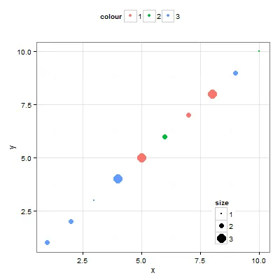
    ### Step 4
# Arrange the three components (plot, leg1, leg2)
# The two legends are positioned outside the plot: 
# one at the top and the other to the side.
plotNew <- arrangeGrob(leg1, plot, 
         heights = unit.c(leg1$height, unit(1, "npc") - leg1$height), ncol = 1)

plotNew <- arrangeGrob(plotNew, leg2,
          widths = unit.c(unit(1, "npc") - leg2$width, leg2$width), nrow = 1)

grid.newpage()
grid.draw(plotNew)

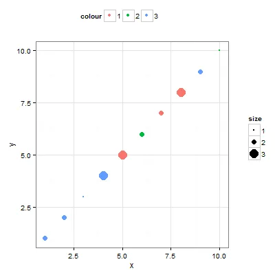
# OR, arrange one legend at the top and the other inside the plot.
plotNew <- plot + 
        annotation_custom(grob = leg2, xmin = 7, xmax = 10, ymin = 0, ymax = 4)

plotNew <- arrangeGrob(leg1, plotNew,
     heights = unit.c(leg1$height, unit(1, "npc") -  leg1$height), ncol = 1)

grid.newpage()
grid.draw(plotNew)

- Sandy Muspratt

---

嗨，Sandy。这是一个令人印象深刻的例子。你能分解一下在arrangeGrob中使用heights参数的逻辑吗？例如，在plotNew <- arrangeGrob(leg1, plot, heights = unit.c(leg1$height, unit(1, "npc") - leg1$height), ncol = 1)中。我知道heights作为参数传递给了grid.layout，但我很难看出它在这里的用法。谢谢。 - Faheem Mitha

这是另一个相关的后续，这是GitHub问题：在某些情况下多次调用annotation_custom失败。 Sandy，我很感激如果您能告诉我是否可以重现。 - Faheem Mitha

@FaheemMitha 我能复现你的问题。一段时间以前，我也遇到了类似的问题。使用annotation_custom，我可以定位多个表格、文本、线条、矩形等，但无法定位多个图形。我的解决方法是使用视口(viewports)，并改编自 http://stackoverflow.com/questions/10539376/10539376。 - Sandy Muspratt

谢谢，Sandy。我认为修复错误比绕过它们更好，但这可能很困难。我已经对问题进行了一些分析，尽管我在后面的部分所关注的可能是一个不相关的错误。 - Faheem Mitha

这仍然是实现此目标的最佳方法吗？只是想检查一下，因为自原答案发布以来已经过去了约8年，自最近的编辑以来已经过去了约5年。 - C.Robin

Answer 2

使用 ggplot2 和 cowplot（= ggplot2扩展）。

这种方法与Sandy的方法类似，它将图例作为单独的对象提取出来，并让您可以独立地进行放置。它主要设计用于属于网格中两个或多个绘图的多个图例。

思路如下：

1. 创建带有没有图例的Plot1、Plot2、...、PlotX
2. 创建带有有图例的Plot1、Plot2、...、PlotX
3. 从步骤1和2中提取图例并放入单独的对象中
4. 设置图例网格并按照您想要的方式排列图例
5. 创建组合绘图和图例的网格

看起来有点复杂和耗费时间/代码，但是只需设置一次，您就可以适应并将其用于各种类型的绘图/图例自定义。

library(ggplot2)
library(cowplot)

# Some data
df <- data.frame(
  Name = factor(rep(c("A", "B", "C"), 12)),
  Month = factor(rep(1:12, each = 3)),
  Temp = sample(0:40, 12),
  Precip = sample(50:400, 12)
)

# 1. create plot1
plot1 <- ggplot(df, aes(Month, Temp, fill = Name)) +
  geom_point(
    show.legend = F, aes(group = Name, colour = Name),
    size = 3, shape = 17
  ) +
  geom_smooth(
    method = "loess", se = F,
    aes(group = Name, colour = Name),
    show.legend = F, size = 0.5, linetype = "dashed"
  )

# 2. create plot2
plot2 <- ggplot(df, aes(Month, Precip, fill = Name)) +
  geom_bar(stat = "identity", position = "dodge", show.legend = F) +
  geom_smooth(
    method = "loess", se = F,
    aes(group = Name, colour = Name),
    show.legend = F, size = 1, linetype = "dashed"
  ) +
  scale_fill_grey()

# 3.1 create legend1
legend1 <- ggplot(df, aes(Month, Temp)) +
  geom_point(
    show.legend = T, aes(group = Name, colour = Name),
    size = 3, shape = 17
  ) +
  geom_smooth(
    method = "loess", se = F, aes(group = Name, colour = Name),
    show.legend = T, size = 0.5, linetype = "dashed"
  ) +
  labs(colour = "Station") +
  theme(
    legend.text = element_text(size = 8),
    legend.title = element_text(
      face = "italic",
      angle = -0, size = 10
    )
  )

# 3.2 create legend2
legend2 <- ggplot(df, aes(Month, Precip, fill = Name)) +
  geom_bar(stat = "identity", position = "dodge", show.legend = T) +
  scale_fill_grey() +
  guides(
    fill =
      guide_legend(
        title = "",
        title.theme = element_text(
          face = "italic",
          angle = -0, size = 10
        )
      )
  ) +
  theme(legend.text = element_text(size = 8))

# 3.3 extract "legends only" from ggplot object
legend1 <- get_legend(legend1)
legend2 <- get_legend(legend2)

# 4.1 setup legends grid
legend1_grid <- cowplot::plot_grid(legend1, align = "v", nrow = 2)

# 4.2 add second legend to grid, specifying its location
legends <- legend1_grid +
  ggplot2::annotation_custom(
    grob = legend2,
    xmin = 0.5, xmax = 0.5, ymin = 0.55, ymax = 0.55
  )

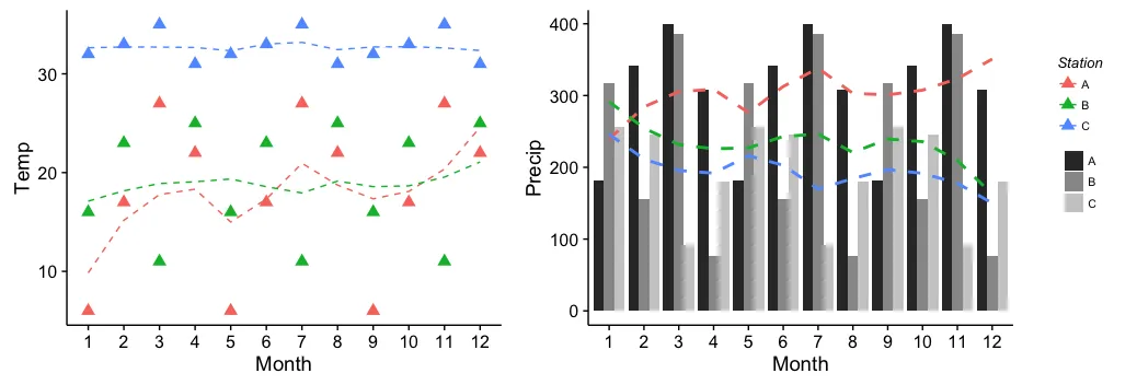
# 5. plot "plots" + "legends" (with legends in between plots)
cowplot::plot_grid(plot1, legends, plot2,
  ncol = 3,
  rel_widths = c(0.45, 0.1, 0.45)
)

^{这是由reprex package（v0.3.0）于2019年10月5日创建的。}

---

将最后一个 plot_grid() 的调用顺序改变可以将图例移动到右侧：

cowplot::plot_grid(plot1, plot2, legends, ncol = 3, 
                   rel_widths = c(0.45, 0.45, 0.1))

- pat-s

Answer 3

据我了解，在ggplot2中对图例的控制非常有限。以下是Hadley的书中的一段话（第111页）：

ggplot2试图使用最少的图例来准确传达绘图中使用的美学特征。如果一个变量与多个美学特征一起使用，则通过合并图例来实现。图6.14展示了这种情况的一个示例：如果颜色和形状都映射到同一个变量，则只需要一个图例。为了合并图例，它们必须具有相同的名称（相同的图例标题）。因此，如果更改合并后的任何一个图例的名称，则需要为所有图例更改名称。

- alittleboy

---

感谢提取。所有示例都显示相同位置的图例。 - pssguy