我使用了其中一个提出的算法,但结果非常糟糕。
我在Java中实现了维基算法(代码如下)。
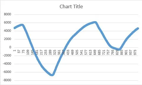
我得到的结果如下: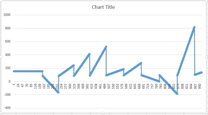 但应该与这个类似:
 同时,我也试图按照http://www.geos.ed.ac.uk/~yliu23/docs/lect_spline.pdf中的方式以另一种方法实现算法。
首先他们展示了如何进行线性样条插值,这很容易。我创建了计算A和B系数的函数。然后他们通过添加二阶导数来扩展线性样条插值。C和D系数也很容易计算。
但是当我尝试计算二阶导数时,问题就开始了。我不知道他们是如何计算的。
因此,我只实现了线性插值。结果如下: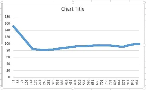 有人知道如何修复第一个算法或者解释一下第二个算法中如何计算二阶导数吗?
我在Java中实现了维基算法(代码如下)。
x(0)是points.get(0),y(0)是values[points.get(0)],α是alfa,μ是mi。其余部分与维基伪代码相同。 public void createSpline(double[] values, ArrayList<Integer> points){
a = new double[points.size()+1];
for (int i=0; i <points.size();i++)
{
a[i] = values[points.get(i)];
}
b = new double[points.size()];
d = new double[points.size()];
h = new double[points.size()];
for (int i=0; i<points.size()-1; i++){
h[i] = points.get(i+1) - points.get(i);
}
alfa = new double[points.size()];
for (int i=1; i <points.size()-1; i++){
alfa[i] = (double)3 / h[i] * (a[i+1] - a[i]) - (double)3 / h[i-1] *(a[i+1] - a[i]);
}
c = new double[points.size()+1];
l = new double[points.size()+1];
mi = new double[points.size()+1];
z = new double[points.size()+1];
l[0] = 1; mi[0] = z[0] = 0;
for (int i =1; i<points.size()-1;i++){
l[i] = 2 * (points.get(i+1) - points.get(i-1)) - h[i-1]*mi[i-1];
mi[i] = h[i]/l[i];
z[i] = (alfa[i] - h[i-1]*z[i-1])/l[i];
}
l[points.size()] = 1;
z[points.size()] = c[points.size()] = 0;
for (int j=points.size()-1; j >0; j--)
{
c[j] = z[j] - mi[j]*c[j-1];
b[j] = (a[j+1]-a[j]) - (h[j] * (c[j+1] + 2*c[j])/(double)3) ;
d[j] = (c[j+1]-c[j])/((double)3*h[j]);
}
for (int i=0; i<points.size()-1;i++){
for (int j = points.get(i); j<points.get(i+1);j++){
// fk[j] = values[points.get(i)];
functionResult[j] = a[i] + b[i] * (j - points.get(i))
+ c[i] * Math.pow((j - points.get(i)),2)
+ d[i] * Math.pow((j - points.get(i)),3);
}
}
}
我得到的结果如下:
但应该与这个类似:
同时,我也试图按照http://www.geos.ed.ac.uk/~yliu23/docs/lect_spline.pdf中的方式以另一种方法实现算法。首先他们展示了如何进行线性样条插值,这很容易。我创建了计算A和B系数的函数。然后他们通过添加二阶导数来扩展线性样条插值。C和D系数也很容易计算。
但是当我尝试计算二阶导数时,问题就开始了。我不知道他们是如何计算的。
因此,我只实现了线性插值。结果如下:
有人知道如何修复第一个算法或者解释一下第二个算法中如何计算二阶导数吗?