首先,绝不要做这样的事情:
mat = []
X = []
Y = []

for x in range(0,bignum):
    mat.append([])
    X.append(x);
    for y in range (0,bignum):
        mat[x].append(random.random())
        Y.append(y)
这等同于:
mat = np.random.random((bignum, bignum))
X, Y = np.mgrid[:bignum, :bignum]
... 但它比使用列表并转换为数组要快数个数量级,并且使用的内存只是一小部分。
然而,你的示例完美地运行了。
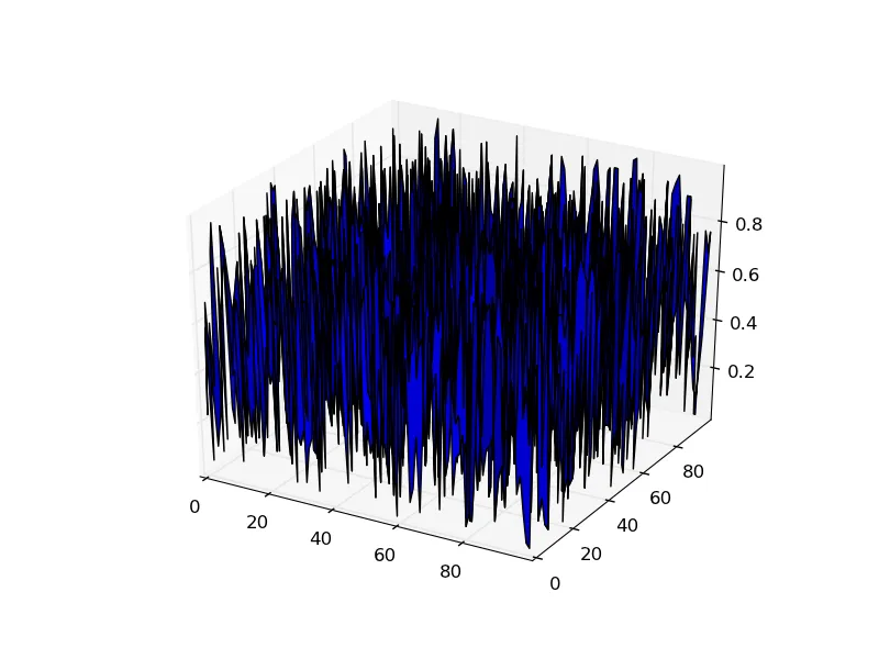
from mpl_toolkits.mplot3d import Axes3D
import matplotlib.pyplot as plt
import numpy as np

bignum = 100
mat = np.random.random((bignum, bignum))
X, Y = np.mgrid[:bignum, :bignum]

fig = plt.figure()
ax = fig.add_subplot(1,1,1, projection='3d')
surf = ax.plot_surface(X,Y,mat)
plt.show()
如果你阅读了plot_surface的文档,就会发现X、Y和Z应该是二维数组。
这样做是为了能够通过隐式定义点之间的连接来绘制更复杂的曲面(例如球体)。 (例如,可以参考matplotlib图库中的这个例子:http://matplotlib.sourceforge.net/examples/mplot3d/surface3d_demo2.html)
如果你有一维的X和Y数组,并希望从二维网格得到简单的曲面,则使用numpy.meshgrid或numpy.mgrid生成相应的X和Y二维数组。
编辑:
只是为了解释mgrid和meshgrid的作用,让我们看一下它们的输出:
print np.mgrid[:5, :5]
产生:
array([[[0, 0, 0, 0, 0],
        [1, 1, 1, 1, 1],
        [2, 2, 2, 2, 2],
        [3, 3, 3, 3, 3],
        [4, 4, 4, 4, 4]],

       [[0, 1, 2, 3, 4],
        [0, 1, 2, 3, 4],
        [0, 1, 2, 3, 4],
        [0, 1, 2, 3, 4],
        [0, 1, 2, 3, 4]]])
所以,它返回一个形状为2x5x5的单一3D数组,但更容易将其视为两个2D数组。其中一个表示5x5网格上任意点的
i坐标,而另一个表示
j坐标。
由于Python解包的工作方式,我们可以直接写:
xx, yy = np.mgrid[:5, :5]
Python不关心mgrid返回的具体内容,它只会尝试将其解包为两个条目。因为numpy数组在它们的第一个轴上迭代切片,如果我们解包具有形状(2x5x5)的数组,我们将得到2个大小为5x5的数组。类似地,我们可以做一些像这样的事情:
xx, yy, zz = np.mgrid[:5, :5, :5]
从stackoverflow获取而来,我们可以使用np.mgrid函数获得3个数组,它们都是5x5x5的索引矩阵。如果我们使用不同的范围(例如xx, yy = np.mgrid[10:15, 3:8])进行切片,它将会在10到14以及3到7的区间内重复索引。
mgrid还有一些其他的功能(例如可以使用复合步骤参数模拟linspace。例如:xx, yy = np.mgrid[0:1:10j, 0:5:5j]将返回两个分别在0-1和0-5之间递增的大小为10x5的数组),但是我们现在先跳过这些内容,继续介绍meshgrid。
meshgrid函数也会将两个数组进行类似于mgrid的扩展操作。例如:
x = np.arange(5)
y = np.arange(5)
xx, yy = np.meshgrid(x, y)
print xx, yy
产出:
(array([[0, 1, 2, 3, 4],
       [0, 1, 2, 3, 4],
       [0, 1, 2, 3, 4],
       [0, 1, 2, 3, 4],
       [0, 1, 2, 3, 4]]),

array([[0, 0, 0, 0, 0],
       [1, 1, 1, 1, 1],
       [2, 2, 2, 2, 2],
       [3, 3, 3, 3, 3],
       [4, 4, 4, 4, 4]]))
meshgrid实际上返回了一个包含两个元素的元组,每个元素都是一个5x5的二维数组,但这种区别并不重要。关键的区别在于索引值不必朝特定方向递增,它只是将给定的数组进行平铺。例如:
x = [0.1, 2.4, -5, 19]
y = [-4.3, 2, -1, 18.4]
xx, yy = np.meshgrid(x, y)
产生:
(array([[  0.1,   2.4,  -5. ,  19. ],
       [  0.1,   2.4,  -5. ,  19. ],
       [  0.1,   2.4,  -5. ,  19. ],
       [  0.1,   2.4,  -5. ,  19. ]]),
 array([[ -4.3,  -4.3,  -4.3,  -4.3],
       [  2. ,   2. ,   2. ,   2. ],
       [ -1. ,  -1. ,  -1. ,  -1. ],
       [ 18.4,  18.4,  18.4,  18.4]]))
你会注意到,它只是将我们提供的值平铺。
基本上,当你需要使用与输入网格相同形状的索引时,就可以使用它们。 当您想要在网格值上评估函数时,这通常非常有用。
例如:
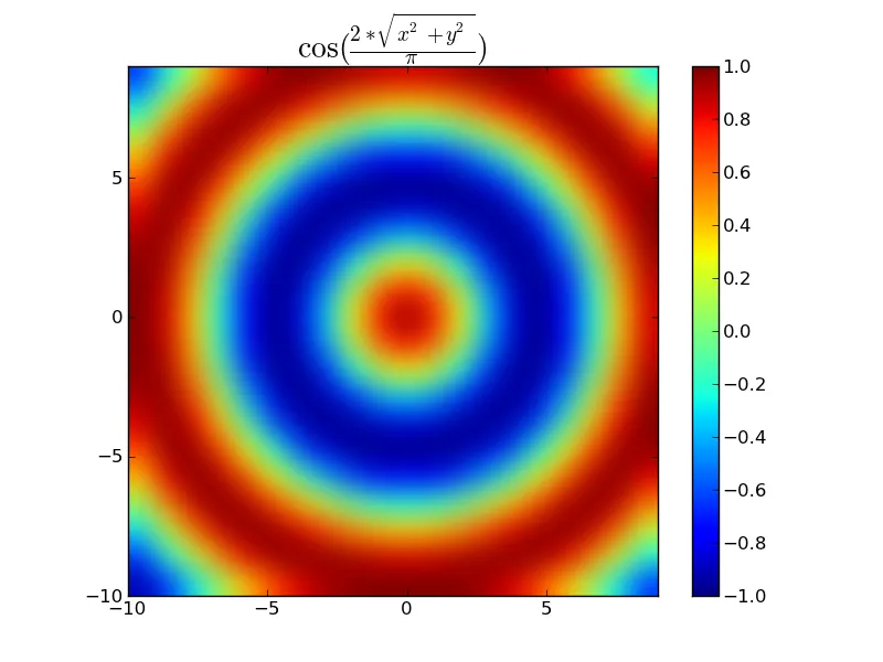
import numpy as np
import matplotlib.pyplot as plt
x, y = np.mgrid[-10:10, -10:10]
dist = np.hypot(x, y)
z = np.cos(2 * dist / np.pi)
plt.title(r'$\cos(\frac{2*\sqrt{x^2 + y^2}}{\pi})$', size=20)
plt.imshow(z, origin='lower', interpolation='bicubic',
extent=(x.min(), x.max(), y.min(), y.max()))
plt.colorbar()
plt.show()