我一直试图找到在六边形散点图上添加loess回归线的方法。目前为止,我没有任何成功... 有什么建议吗?
我的代码如下:
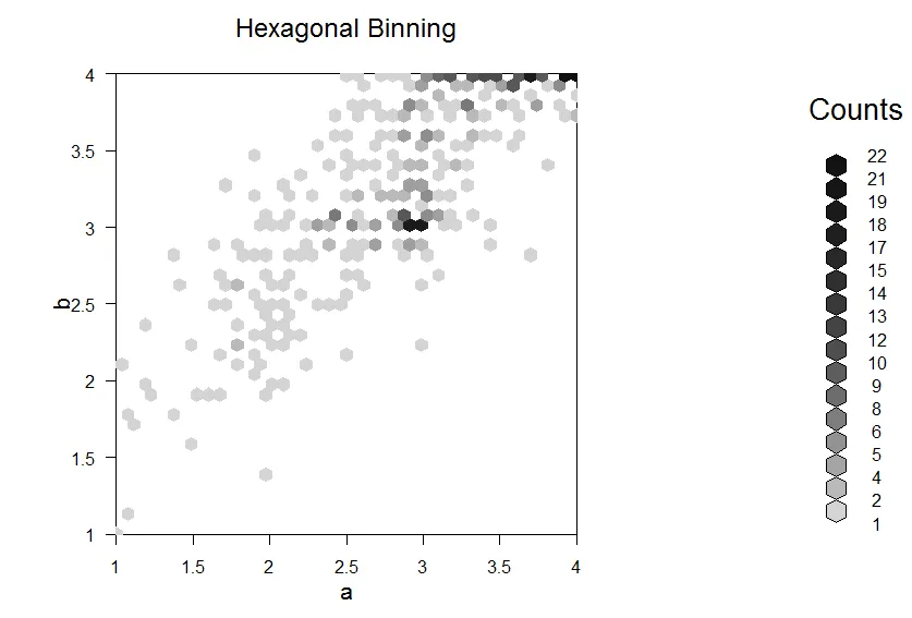
bin<-hexbin(Dataset$a, Dataset$b, xbins=40)

plot(bin, main="Hexagonal Binning",
     xlab = "a", ylab = "b",
     type="l")
我一直试图找到在六边形散点图上添加loess回归线的方法。目前为止,我没有任何成功... 有什么建议吗?
我的代码如下:
bin<-hexbin(Dataset$a, Dataset$b, xbins=40)
plot(bin, main="Hexagonal Binning",
xlab = "a", ylab = "b",
type="l")
ggplot2来绘制图表。palmerpenguins包数据集。library(palmerpenguins) # For the data
library(ggplot2) # ggplot2 for plotting
ggplot(penguins, aes(x = body_mass_g,
y = bill_length_mm)) +
geom_hex(bins = 40) +
geom_smooth(method = 'loess', se = F, color = 'red')

该文本创建于2021年1月5日,使用reprex包(v0.3.0)
我没有针对base的解决方案,但是可以使用ggplot来实现。使用base也应该是可能的,但是如果您查看?hexbin的文档,您会看到以下引用:
请注意,在绘制hexbin对象时,使用grid软件包。您必须使用其图形(或如果您知道如何使用lattice软件包)添加到此类情节中。
我不熟悉如何修改这些内容。我尝试使用ggplotify将base转换为ggplot,并以此方式进行编辑,但无法正确地将loess线添加到绘图窗口中。
因此,这里提供了一个解决方案,使用一些虚假数据,您可以在Datasets上尝试:
library(hexbin)
library(ggplot2)

# fake data with a random walk, replace with your data
set.seed(100)
N <- 1000
x <- rnorm(N)
x <- sort(x)
y <- vector("numeric", length=N)
for(i in 2:N){
  y[i] <- y[i-1] + rnorm(1, sd=0.1)
}

# current method
# In documentation for ?hexbin it says:
# "You must use its graphics (or those from package lattice if you know how) to add to such plots."
(bin <- hexbin(x, y, xbins=40))
plot(bin)

# ggplot option. Can play around with scale_fill_gradient to
# get the colour scale similar or use other ggplot options
df <- data.frame(x=x, y=y)
d <- ggplot(df, aes(x, y)) +
  geom_hex(bins=40) +
  scale_fill_gradient(low = "grey90", high = "black") +
  theme_bw()
d

# easy to add a loess fit to the data
# span controls the degree of smoothing, decrease to make the line
# more "wiggly"
model <- loess(y~x, span=0.2)
fit <- predict(model)
loess_data <- data.frame(x=x, y=fit)
d + geom_line(data=loess_data, aes(x=x, y=y), col="darkorange",
              size=1.5)
这里有两个选项;您需要决定是对原始数据进行平滑处理还是对分组数据进行平滑处理。
library(hexbin)
library(grid)

# Some data
set.seed(101)
d <- data.frame(x=rnorm(1000))
d$y <- with(d, 2*x^3 + rnorm(1000))
方法A - 分组数据
# plot hexbin & smoother : need to grab plot viewport
# From ?hexVP.loess : "Fit a loess line using the hexagon centers of mass
# as the x and y coordinates and the cell counts as weights."
bin <- hexbin(d$x, d$y)
p <- plot(bin)
hexVP.loess(bin, hvp = p$plot.vp, span = 0.4, col = "red", n = 200)
# calculate loess predictions outside plot on raw data
l = loess(y ~ x, data=d, span=0.4)
xp = with(d, seq(min(x), max(x), length=200))
yp = predict(l, xp)

# plot hexbin
bin <- hexbin(d$x, d$y)
p <- plot(bin)

# add loess line
pushHexport(p$plot.vp)
grid.lines(xp, yp, gp=gpar(col="red"), default.units = "native")
upViewport()