使用
get_forecast() 方法可以得到时间序列结果,从而获得更加平滑的图形。以下是时间序列的示例:
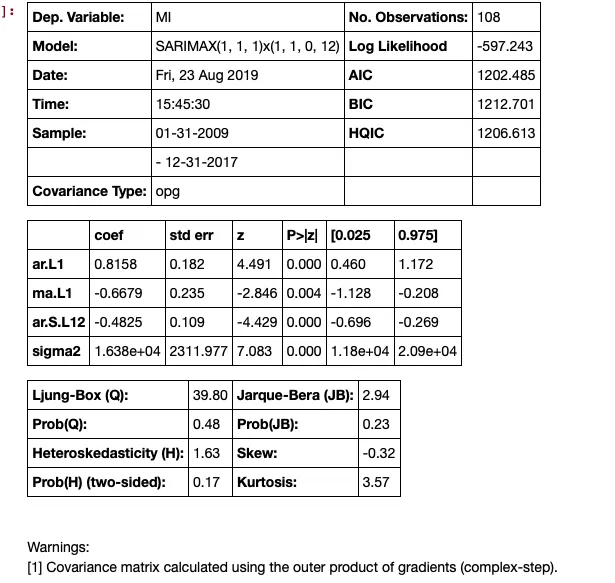
model = SARIMAX(train['MI'], order=(1,1,1), seasonal_order=(1,1,0,12), enforce_invertibility=True)
results = model.fit()
results.summary()
下一步是进行预测,这将生成置信区间。
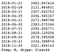
predictions_int = results.get_forecast(steps=11)
predictions_int.predicted_mean
这些可以放在数据框中,但需要进行一些清理:
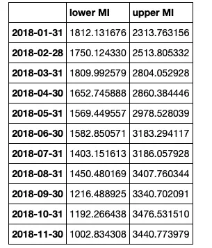
predictions_int.conf_int()
将数据框连接起来,但清理表头
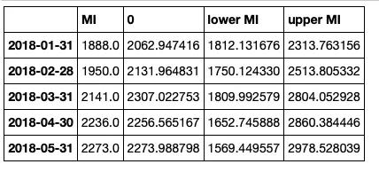
conf_df = pd.concat([test['MI'],predictions_int.predicted_mean, predictions_int.conf_int()], axis = 1)

conf_df.head()
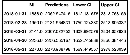
然后我们重命名列。
conf_df = conf_df.rename(columns={0: 'Predictions', 'lower MI': 'Lower CI', 'upper MI': 'Upper CI'})
conf_df.head()
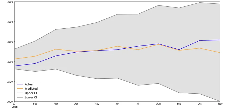
制作图表。
# make a plot of model fit
# color = 'skyblue'

fig = plt.figure(figsize = (16,8))
ax1 = fig.add_subplot(111)


x = conf_df.index.values


upper = conf_df['Upper CI']
lower = conf_df['Lower CI']

conf_df['MI'].plot(color = 'blue', label = 'Actual')
conf_df['Predictions'].plot(color = 'orange',label = 'Predicted' )
upper.plot(color = 'grey', label = 'Upper CI')
lower.plot(color = 'grey', label = 'Lower CI')

# plot the legend for the first plot
plt.legend(loc = 'lower left', fontsize = 12)


# fill between the conf intervals
plt.fill_between(x, lower, upper, color='grey', alpha='0.2')

plt.ylim(1000,3500)

plt.show()