我需要一个算法,可以为N个点(可能少于20个)在球体周围提供位置,并使它们大致分散。没有必要“完美”,但我只需要确保它们不会聚集在一起。
几个我遇到的问题线程提到了随机均匀分布,这增加了我不关心的复杂度。我很抱歉这是一个愚蠢的问题,但我想表明我真的很努力地寻找答案,但仍然没有结果。
所以,我要找的是简单的伪代码,用于在单位球周围均匀分布N个点,可以返回球面或笛卡尔坐标。如果它能够稍微随机分布(考虑行星绕恒星运行,相当分散,但有余地),那就更好了。
在球面上均匀分布n个点
193
- Befall
5
你说的“加入一点随机性”是什么意思?你是指在某种程度上进行扰动吗? - ninjagecko
43OP很困惑。他想在球体上放置n个点,使得任意两点之间的最小距离尽可能大。这将使这些点看起来“均匀地分布”在整个球体上。这与创建球面上的均匀随机分布完全无关,这是那些链接所涉及的内容,也是下面许多答案所谈论的内容。 - BlueRaja - Danny Pflughoeft
1如果您不希望点看起来随意分布,那么在球体上放置20个点并不算很多。 - John Alexiou
2这里有一种方法可以实现它(其中包含代码示例):https://pdfs.semanticscholar.org/97a6/7e367e39762baf631f519c00fbfd1d5c009a.pdf(看起来似乎使用了排斥力计算)。 - trusktr
2当N的取值为{4,6,8,12,20}时,显然存在精确解,其中每个点到其最近邻的距离对于所有点和所有最近邻都是恒定的。 - dmckee --- ex-moderator kitten
18个回答
222
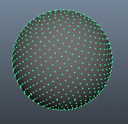
斐波那契球面算法非常适合这个问题。它快速且结果一眼看去很容易欺骗人眼。您可以查看使用processing完成的示例,它将随着点的添加而显示结果。这是@gman制作的另一个出色的交互式示例。这里还有一个简单的Python实现。
import math


def fibonacci_sphere(samples=1000):

    points = []
    phi = math.pi * (math.sqrt(5.) - 1.)  # golden angle in radians

    for i in range(samples):
        y = 1 - (i / float(samples - 1)) * 2  # y goes from 1 to -1
        radius = math.sqrt(1 - y * y)  # radius at y

        theta = phi * i  # golden angle increment

        x = math.cos(theta) * radius
        z = math.sin(theta) * radius

        points.append((x, y, z))

    return points
1000个样本会给你这个结果:
- Fnord
20
1在定义phi时,变量n被调用:phi = ((i + rnd) % n) * increment。n是否等于samples? - Andrew Staroscik
7该代码生成了单位球面上的点,因此只需将每个点乘以所需半径的标量即可。 - Fnord
4@Fnord: 我们能否将此方法用于更高维度的问题? - pikachuchameleon
2真的很酷!!!你用什么工具生成了那个渲染图? - Ferdinando Randisi
显示剩余15条评论
191
黄金螺旋法
你说你无法使用黄金螺旋法,这真是可惜,因为它非常好。我想给你一个完整的了解,这样也许你就能明白如何避免“挤在一起”的情况。
下面是一个快速的、非随机的方法来创建一个近似正确的格子;正如上文所述,没有哪个格子会是完美的,但这可能已经足够了。与其他方法(例如 BendWavy.org)相比,它看起来漂亮,并保证在极限情况下间距均匀。
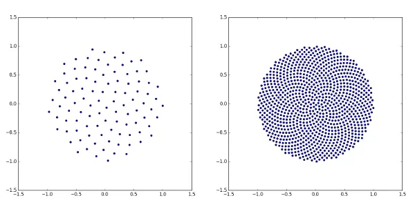
入门:单位圆上的向日葵螺旋
为了理解这个算法,首先请看2D向日葵螺旋算法。它基于一个事实,即最无理数就是黄金比例(1 + sqrt(5))/2,如果以“站在中心,转黄金比例圈,然后朝那个方向发射另一个点”的方式发射点,就会自然地构建一个螺旋形状,随着您增加更多的点数,它仍然拒绝具有明确定义的'条纹',使得点不排成一条线。(注1.)
均匀分布在圆盘上的算法如下:from numpy import pi, cos, sin, sqrt, arange
import matplotlib.pyplot as pp
num_pts = 100
indices = arange(0, num_pts, dtype=float) + 0.5
r = sqrt(indices/num_pts)
theta = pi * (1 + 5**0.5) * indices
pp.scatter(r*cos(theta), r*sin(theta))
pp.show()
它产生的结果看起来像这样(n=100和n=1000):
将点径向分布
关键的奇怪之处在于公式r = sqrt(indices / num_pts);我是如何得出这个公式的?(注2.)
嗯,我在这里使用平方根,因为我希望它们在圆盘周围具有均匀的面积间隔。也就是说,在大的N的极限情况下,我希望一个小区域R ∈ (r, r + dr),Θ ∈ (θ, θ + dθ) 包含的点数与其面积成比例,即r dr dθ。现在,如果我们假装这里涉及到一个随机变量,那么这就有一个简单的解释,即(R,Θ)的联合概率密度仅为c r,其中c是某个常数。在单位圆上的归一化会强制c = 1/π。
现在让我介绍一个技巧。它来自概率论中被称为逆转换采样的方法:假设你想要生成一个具有概率密度函数f(z)的随机变量,并且你有一个随机变量U ~ Uniform(0,1),就像大多数编程语言中的random()函数一样。你该如何实现呢?
- 首先,将你的密度转化为累积分布函数或CDF,我们称之为F(z)。记住,CDF从0单调递增到1,导数为f(z)。
- 然后计算CDF的反函数F-1(z)。
- 你会发现Z=F-1(U)的分布符合目标密度。(注3)
r = sqrt(random()); theta = 2 * pi * random()在极坐标下生成圆盘上的随机点。现在,我们不再对这个反函数进行随机采样,而是进行均匀采样。均匀采样的好处是,当 N 很大时,关于点分布的结果将表现得好像我们已经进行了随机采样。这种组合就是诀窍。我们使用
(arange(0, num_pts, dtype=float) + 0.5)/num_pts 而不是 random(),例如,如果我们要采样10个点,则它们为 r = 0.05, 0.15, 0.25, ... 0.95。我们均匀采样r以获得等面积间距,并使用向日葵增量来避免输出中可怕的“条”形点。
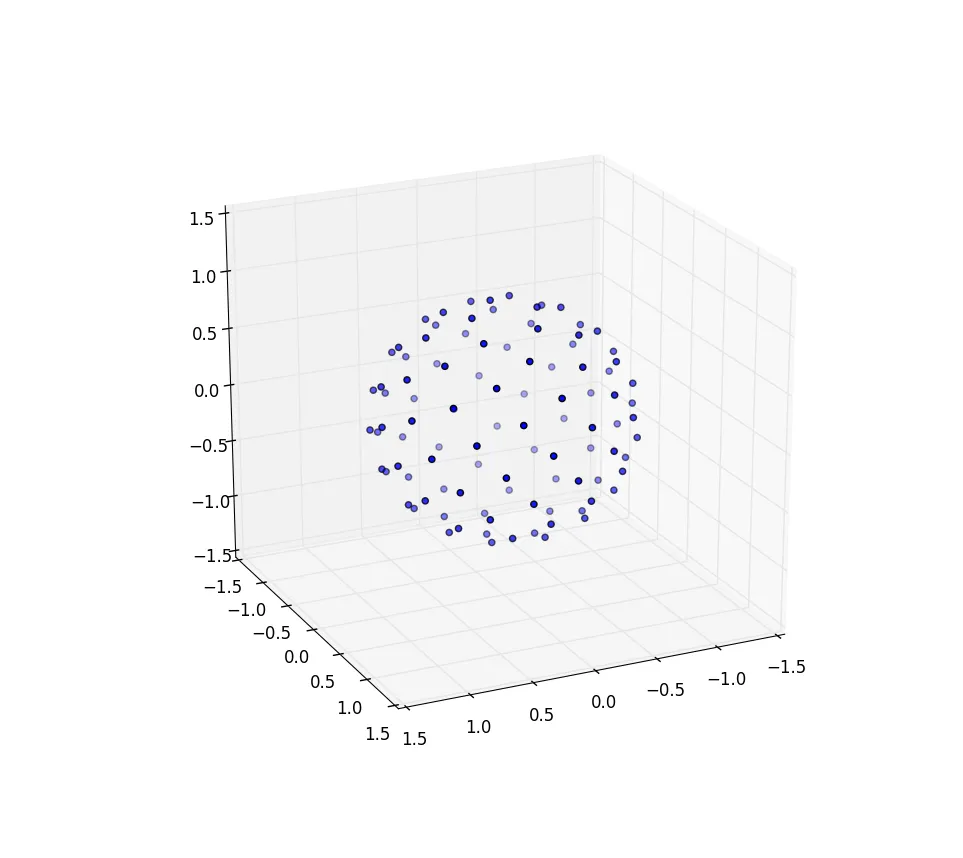
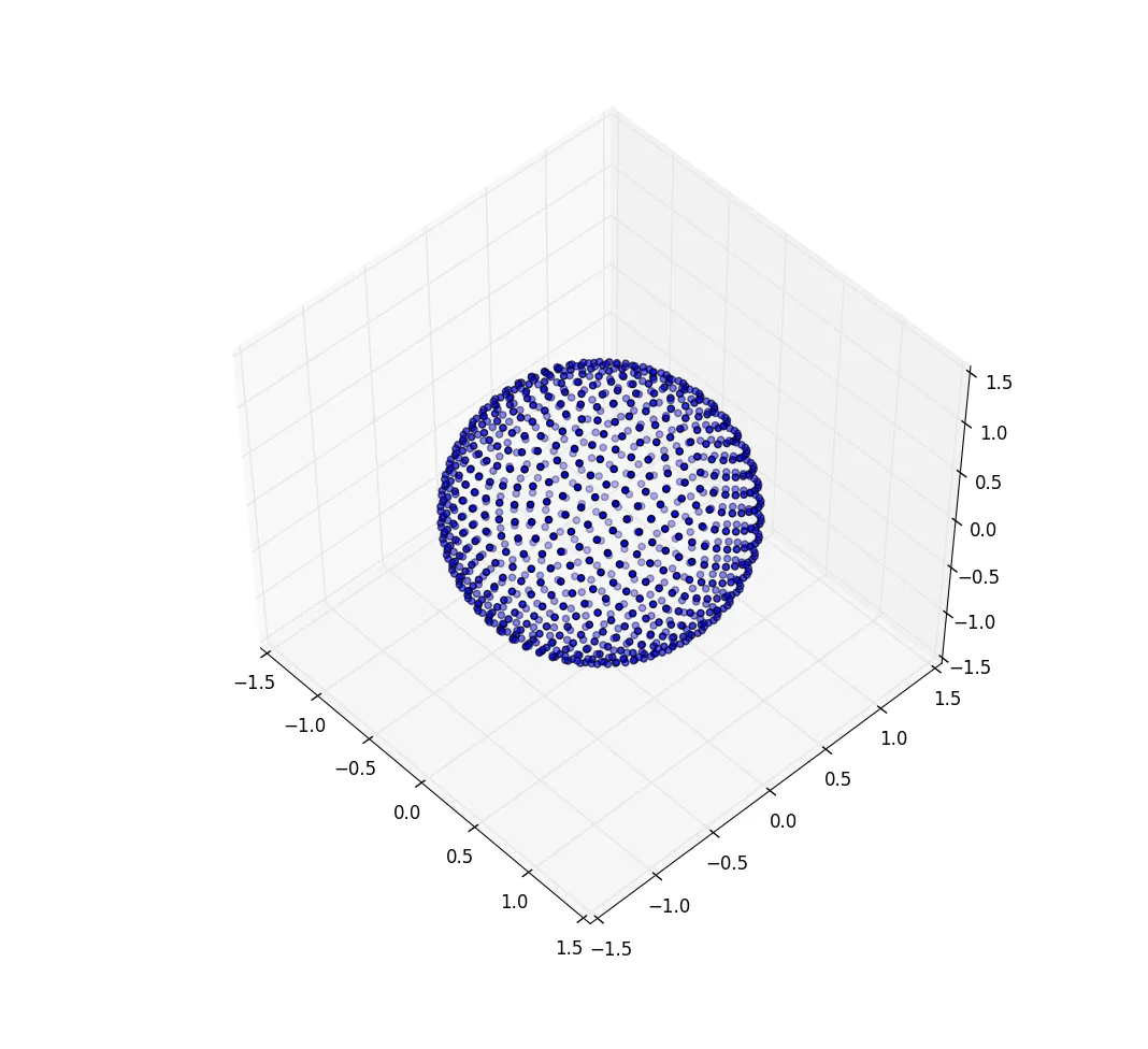
现在在球体上进行向日葵操作
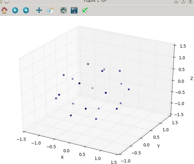
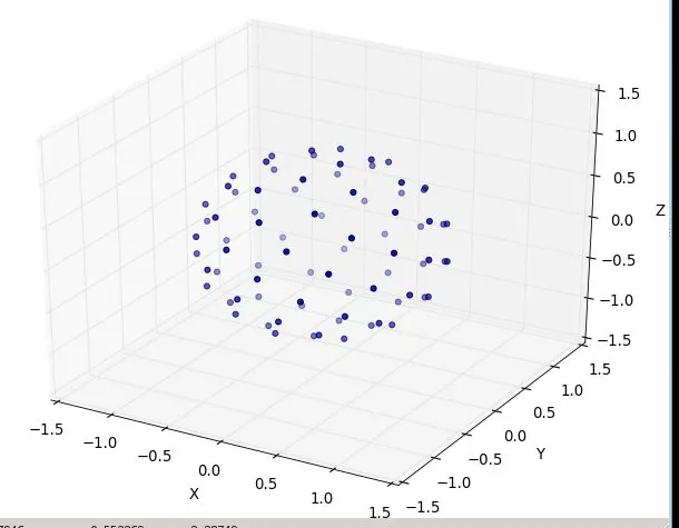
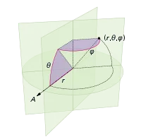
我们需要做的改变只是将极坐标换成球面坐标,以在球面上画点。由于我们在单位球上,径向坐标当然不会进入其中。为了保持一致性,尽管我接受物理学训练,但我将使用数学家的坐标系,其中 0 ≤ φ ≤ π 是从极点下降的纬度,而 0 ≤ θ ≤ 2π 是经度。因此,与上面的区别在于我们基本上用 φ 替换了变量 r。我们的面积元素,原本是rdrdθ,现在变成了不那么复杂的sin(φ)dφdθ。因此,我们均匀间隔的联合密度为sin(φ)/4π。将θ积分,我们得到f(φ)=sin(φ)/2,因此F(φ)=(1-cos(φ))/2。反演后,我们可以看到均匀随机变量看起来像acos(1-2 u),但我们进行的是均匀采样而不是随机采样,因此我们使用φk=acos(1-2 (k+0.5)/N)。算法的其余部分只是将其投影到x、y和z坐标上:
from numpy import pi, cos, sin, arccos, arange
import mpl_toolkits.mplot3d
import matplotlib.pyplot as pp

num_pts = 1000
indices = arange(0, num_pts, dtype=float) + 0.5

phi = arccos(1 - 2*indices/num_pts)
theta = pi * (1 + 5**0.5) * indices

x, y, z = cos(theta) * sin(phi), sin(theta) * sin(phi), cos(phi);

pp.figure().add_subplot(111, projection='3d').scatter(x, y, z);
pp.show()
对于n=100和n=1000的情况,结果如下所示:
进一步研究
我想向马丁·罗伯茨的博客致敬。请注意,我通过给每个索引加上0.5来创建偏移量。这只是出于视觉上的吸引力,但是偏移量的选择很重要,并且在区间内不是恒定的,如果选择正确,可以获得高达8%更好的装箱精度。还应该有一种方法使他的R2序列覆盖一个球体,并且有趣的是看看这是否也产生了漂亮均匀的覆盖,可能是原样,但可能需要从只有一个对角线切割的单位正方形的一半中取出来并拉伸以获取圆形。注释
Those “bars” are formed by rational approximations to a number, and the best rational approximations to a number come from its continued fraction expression,
z + 1/(n_1 + 1/(n_2 + 1/(n_3 + ...)))wherezis an integer andn_1, n_2, n_3, ...is either a finite or infinite sequence of positive integers:def continued_fraction(r): while r != 0: n = floor(r) yield n r = 1/(r - n)Since the fraction part
1/(...)is always between zero and one, a large integer in the continued fraction allows for a particularly good rational approximation: “one divided by something between 100 and 101” is better than “one divided by something between 1 and 2.” The most irrational number is therefore the one which is1 + 1/(1 + 1/(1 + ...))and has no particularly good rational approximations; one can solve φ = 1 + 1/φ by multiplying through by φ to get the formula for the golden ratio.For folks who are not so familiar with NumPy -- all of the functions are “vectorized,” so that
sqrt(array)is the same as what other languages might writemap(sqrt, array). So this is a component-by-componentsqrtapplication. The same also holds for division by a scalar or addition with scalars -- those apply to all components in parallel.The proof is simple once you know that this is the result. If you ask what's the probability that z < Z < z + dz, this is the same as asking what's the probability that z < F-1(U) < z + dz, apply F to all three expressions noting that it is a monotonically increasing function, hence F(z) < U < F(z + dz), expand the right hand side out to find F(z) + f(z) dz, and since U is uniform this probability is just f(z) dz as promised.
- CR Drost
13
5我不确定为什么这么少人知道,这绝对是最好的快速方法。 - Krupip
2@snb 谢谢你的赞美之词!它在这里排名靠后,部分原因是因为它比其他所有答案都要年轻得多。我很惊讶它能够做得这么好。 - CR Drost
2@FelixD。这听起来像是一个问题,如果你开始使用大圆距离而不是欧几里得距离,那么可能会变得非常复杂。但也许我可以回答一个简单的问题,如果将球面上的点转换为它们的 Voronoi 图,那么可以将每个 Voronoi 单元格描述为具有近似面积 4π/N,并且可以通过假装它是一个圆而不是一个菱形来将其转换为特征距离,πr²=4π/N。然后 r=2/√(N)。 - CR Drost
2使用采样定理时,使用实际均匀而不是随机均匀的输入是让我想说“好吧,为什么我没想到呢?”的那种事情。很棒。 - dmckee --- ex-moderator kitten
2很好的问题!我认为我的答案更接近“它起作用的原因”,而马丁的答案则多出了一点精度。黄金比例的定义是满足φ²=φ+1,这可以重新排列为φ-1=1/φ,将其乘以2π时,三角函数会抵消掉第一个数字1。所以在浮点运算中,仅仅减去一个数字1会用0来填充53位,而应该用1来填充。 - CR Drost
显示剩余8条评论
92
这被称为球面点的填充,目前没有(已知的)通用完美解决方案。然而,有许多不完美的解决方案。最流行的三种似乎是:
- 创建模拟。将每个点视为被限制在球体内的电子,然后运行一定步数的模拟。电子之间的排斥会自然地使系统趋向于更稳定的状态,其中各点之间的距离尽可能远。
- 超立方体拒绝采样。这种花哨的方法实际上非常简单:在围绕球体的立方体内均匀选择点(比
n多得多),然后拒绝球外的点。将剩余的点视为向量,并将其归一化。这些是您的“样本”-使用某种方法(随机、贪婪等)选择其中的n个。 - 螺旋逼近。您在球体周围绘制螺旋线,并平均分布点沿着螺旋线。由于涉及到数学问题,这些比模拟更难理解,但速度更快(而且可能涉及更少的代码)。最受欢迎的似乎是由 Saff, et al 提出的方法。
这个问题有here提供更详细的信息。
- BlueRaja - Danny Pflughoeft
7
我将研究安德鲁·库克在下面发布的螺旋策略,但是,您能否请澄清我想要的内容与“均匀随机分布”之间的区别?那只是在球体上完全随机放置点,使它们均匀分布吗?感谢您的帮助。 :) - Befall
4“均匀随机分布”指的是概率分布是均匀的,这意味着在球体上选择一个随机点时,每个点被选中的可能性是相等的。它与点的最终空间分布无关,因此与您的问题无关。 - BlueRaja - Danny Pflughoeft
啊,好的,非常感谢。搜索我的问题导致了大量针对两者的答案,我无法真正理解哪个对我来说是无用的。 - Befall
要明确的是,每个点被选择的概率都为零。在球面上任意两个区域中,点属于这两个区域的概率比等于这两个区域表面积的比例。 - AturSams
2最后一个链接现在已经失效。 - Felix D.
显示剩余2条评论
17
在这个示例代码中,
(换句话说,
或者,以另一种方式构建答案(使用Python):
node[k]表示第k个节点。你正在生成一个包含N个点的数组,而node[k]就是这些点中的第k个(从0到N-1)。如果只有这个让你感到困惑,那么现在你应该可以理解了。(换句话说,
k是一个大小为N的数组,在代码片段开始之前定义,并包含一系列点的列表。)或者,以另一种方式构建答案(使用Python):
> cat ll.py
from math import asin
nx = 4; ny = 5
for x in range(nx):
    lon = 360 * ((x+0.5) / nx)
    for y in range(ny):
        midpt = (y+0.5) / ny
        lat = 180 * asin(2*((y+0.5)/ny-0.5))
        print lon,lat
> python2.7 ll.py
45.0 -166.91313924
45.0 -74.0730322921
45.0 0.0
45.0 74.0730322921
45.0 166.91313924
135.0 -166.91313924
135.0 -74.0730322921
135.0 0.0
135.0 74.0730322921
135.0 166.91313924
225.0 -166.91313924
225.0 -74.0730322921
225.0 0.0
225.0 74.0730322921
225.0 166.91313924
315.0 -166.91313924
315.0 -74.0730322921
315.0 0.0
315.0 74.0730322921
315.0 166.91313924
如果你绘制它,你会发现极地附近的垂直间距更大,以便每个点位于大约相同的空间面积中(在极地附近,"水平"空间较少,因此会多一些"垂直"空间)。
这不同于所有点与其邻居大约具有相同的距离(我认为你的链接谈论的是这个),但可能对你想要的内容足够了,并且改进了简单制作均匀的纬度/经度网格。
- andrew cooke
6
很好,看到数学解决方案感觉不错。我曾考虑使用螺旋线和弧长分离的方法。我仍然不确定如何得到最优解,这是一个有趣的问题。 - Rusty Rob
你看到我编辑了我的答案,在顶部加入了关于node[k]的解释吗?我认为那可能就是你需要的... - andrew cooke
太棒了,感谢您的解释。我现在没有时间,稍后会尝试一下,但非常感谢您帮助我。我会告诉您它对我的目的起到了什么作用。^^ - Befall
使用螺旋方法完美地满足了我的需求,非常感谢您的帮助和澄清。 :) - Befall
你的纬度转换为度数似乎有误。你难道不应该也除以 π 吗? - Ismael Harun
另外,你的纬度计算范围从0到2,这显然是不正确的。也许你想要从中减去1。 - Ismael Harun
13
你要找的东西被称为球形覆盖。球形覆盖问题非常困难,除了少量点数的解决方案外,其它的解决方案都是未知的。已知的一件事是,在球面上给定n个点,总会存在两个距离小于
如果你想用概率方法在球面上生成均匀分布的点,这很容易:通过高斯分布在空间中均匀生成点(Java内置了此功能,而对于其他语言也不难找到代码)。因此,在三维空间中,你需要类似下面的内容:
d = (4-csc^2(\pi n/6(n-2)))^(1/2)的点。如果你想用概率方法在球面上生成均匀分布的点,这很容易:通过高斯分布在空间中均匀生成点(Java内置了此功能,而对于其他语言也不难找到代码)。因此,在三维空间中,你需要类似下面的内容:
Random r = new Random();
double[] p = { r.nextGaussian(), r.nextGaussian(), r.nextGaussian() };
然后通过将点与原点的距离归一化来将其投影到球体上
double norm = Math.sqrt( (p[0])^2 + (p[1])^2 + (p[2])^2 );
double[] sphereRandomPoint = { p[0]/norm, p[1]/norm, p[2]/norm };
在 n 维度中,高斯分布具有球对称性,因此其投影到球面上是均匀的。
当然,并不能保证均匀生成的点集中任意两点之间的距离都被限制在某个下限范围内,所以你可以使用拒绝抽样来强制实现这些约束条件:最好先生成整个集合,如果需要的话再拒绝整个集合(或者使用“早期拒绝”来拒绝到目前为止已经生成的整个集合;只是不要保留一些点而放弃其他点)。您可以使用上述给出的公式减去一些余量,以确定点之间的最小距离,低于这个距离将拒绝一组点。你将不得不计算n选2个距离,并且拒绝的概率将取决于余量;很难说如何,因此运行模拟以了解相关统计数据的情况。
- Edward Doolittle
1
点赞最小最大距离表达式。对于限制您想要使用的点数非常有用。不过,提供一个权威来源的参考会更好。 - dmckee --- ex-moderator kitten
9
This answer is based on the same 'theory' that is outlined well by this answer
I'm adding this answer as:
-- None of the other options fit the 'uniformity' need 'spot-on' (or not obviously-clearly so). (Noting to get the planet like distribution looking behavior particularly wanted in the original ask, you just reject from the finite list of the k uniformly created points at random (random wrt the index count in the k items back).)
-- The closest other impl forced you to decide the 'N' by 'angular axis', vs. just 'one value of N' across both angular axis values (which at low counts of N is very tricky to know what may, or may not matter (e.g. you want '5' points -- have fun))
-- Furthermore, it's very hard to 'grok' how to differentiate between the other options without any imagery, so here's what this option looks like (below), and the ready-to-run implementation that goes with it.
with N at 20:
with N at 20:
然后在80处加入N:
from math import cos, sin, pi, sqrt

def GetPointsEquiAngularlyDistancedOnSphere(numberOfPoints=45):
    """ each point you get will be of form 'x, y, z'; in cartesian coordinates
        eg. the 'l2 distance' from the origion [0., 0., 0.] for each point will be 1.0
        ------------
        converted from:  http://web.archive.org/web/20120421191837/http://www.cgafaq.info/wiki/Evenly_distributed_points_on_sphere )
    """
    dlong = pi*(3.0-sqrt(5.0))  # ~2.39996323
    dz   =  2.0/numberOfPoints
    long =  0.0
    z    =  1.0 - dz/2.0
    ptsOnSphere =[]
    for k in range( 0, numberOfPoints):
        r    = sqrt(1.0-z*z)
        ptNew = (cos(long)*r, sin(long)*r, z)
        ptsOnSphere.append( ptNew )
        z    = z - dz
        long = long + dlong
    return ptsOnSphere

if __name__ == '__main__':
    ptsOnSphere = GetPointsEquiAngularlyDistancedOnSphere( 80)

    #toggle True/False to print them
    if( True ):
        for pt in ptsOnSphere:  print( pt)

    #toggle True/False to plot them
    if(True):
        from numpy import *
        import pylab as p
        import mpl_toolkits.mplot3d.axes3d as p3

        fig=p.figure()
        ax = p3.Axes3D(fig)

        x_s=[];y_s=[]; z_s=[]

        for pt in ptsOnSphere:
            x_s.append( pt[0]); y_s.append( pt[1]); z_s.append( pt[2])

        ax.scatter3D( array( x_s), array( y_s), array( z_s) )
        ax.set_xlabel('X'); ax.set_ylabel('Y'); ax.set_zlabel('Z')
        p.show()
        #end
经过低计数(N为2、5、7、13等)测试,看起来运作良好。
- Matt S.
8
尝试:
function sphere ( N:float,k:int):Vector3 {
    var inc =  Mathf.PI  * (3 - Mathf.Sqrt(5));
    var off = 2 / N;
    var y = k * off - 1 + (off / 2);
    var r = Mathf.Sqrt(1 - y*y);
    var phi = k * inc;
    return Vector3((Mathf.Cos(phi)*r), y, Mathf.Sin(phi)*r);
};
上述函数应在循环中运行,总共有N个循环和k个当前迭代。
它基于向日葵种子的图案,除了向日葵种子弯曲成半圆顶,再弯曲成球体。
这是一张图片,只不过我把相机放在球体的一半里面。
- bandybabboon
5
Healpix解决了一个密切相关的问题(用等面积像素对球体进行像素化):http://healpix.sourceforge.net/。这可能有点过度,但是也许在查看后,您会意识到它的其他良好属性对您很有趣。它远不止是输出点云的功能。我之前在试图找到它时来到这里;"healpix"这个名字并不准确地唤起球形的联想...
- Andrew Wagner
3
编辑:这并没有回答OP想问的问题,但如果人们在某种程度上发现它有用,我会留下它。
我们使用概率的乘法规则,结合无穷小。这将导致两行代码来实现您所需的结果:
longitude: φ = uniform([0,2pi))
azimuth:   θ = -arcsin(1 - 2*uniform([0,1]))
(定义在以下坐标系中:)
您的语言通常具有均匀随机数原语。例如,在Python中,您可以使用random.random()返回范围在[0,1)内的数字。您可以将此数字乘以k以获得[0,k)范围内的随机数。因此,在Python中,uniform([0,2π))表示random.random()* 2 * math.pi。
证明
现在我们不能均匀地分配θ,否则我们会在极点处聚集。我们希望按球面楔形体(此图中的θ实际上是φ)的表面积分配概率:
在赤道处的角位移dφ将导致dφ*r的位移。在任意方位角θ处的位移是多少?嗯,从z轴的半径为r*sin(θ), 因此与楔形相交的“纬度”弧长是dφ* r*sin(θ)。因此,我们通过对从南极到北极的片的面积进行积分来计算采样的累积分布函数(CDF)。
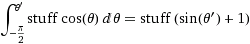 (其中stuff=
dφ*r)
现在我们将尝试获取逆CDF以从中采样:http://en.wikipedia.org/wiki/Inverse_transform_sampling
首先,通过将几乎是CDF的值除以其最大值来进行归一化。这会取消dφ和r的副作用。
azimuthalCDF: cumProb = (sin(θ)+1)/2 from -pi/2 to pi/2

inverseCDF: θ = -sin^(-1)(1 - 2*cumProb)
因此:
let x by a random float in range [0,1]
θ = -arcsin(1-2*x)
- ninjagecko
2
这不就等同于他放弃的“100%随机化”选项吗?我的理解是,他希望它们比均匀随机分布更均匀地分布。 - andrew cooke
1@BlueRaja-DannyPflughoeft:嗯,说得对。我想我没有仔细阅读问题。无论如何,我还是把它留在这里,以防其他人发现它有用。感谢您指出这一点。 - ninjagecko
2
如果点数较少,您可以运行模拟:
from random import random,randint
r = 10
n = 20
best_closest_d = 0
best_points = []
points = [(r,0,0) for i in range(n)]
for simulation in range(10000):
    x = random()*r
    y = random()*r
    z = r-(x**2+y**2)**0.5
    if randint(0,1):
        x = -x
    if randint(0,1):
        y = -y
    if randint(0,1):
        z = -z
    closest_dist = (2*r)**2
    closest_index = None
    for i in range(n):
        for j in range(n):
            if i==j:
                continue
            p1,p2 = points[i],points[j]
            x1,y1,z1 = p1
            x2,y2,z2 = p2
            d = (x1-x2)**2+(y1-y2)**2+(z1-z2)**2
            if d < closest_dist:
                closest_dist = d
                closest_index = i
    if simulation % 100 == 0:
        print simulation,closest_dist
    if closest_dist > best_closest_d:
        best_closest_d = closest_dist
        best_points = points[:]
    points[closest_index]=(x,y,z)


print best_points
>>> best_points
[(9.921692138442777, -9.930808529773849, 4.037839326088124),
 (5.141893371460546, 1.7274947332807744, -4.575674650522637),
 (-4.917695758662436, -1.090127967097737, -4.9629263893193745),
 (3.6164803265540666, 7.004158551438312, -2.1172868271109184),
 (-9.550655088997003, -9.580386054762917, 3.5277052594769422),
 (-0.062238110294250415, 6.803105171979587, 3.1966101417463655),
 (-9.600996012203195, 9.488067284474834, -3.498242301168819),
 (-8.601522086624803, 4.519484132245867, -0.2834204048792728),
 (-1.1198210500791472, -2.2916581379035694, 7.44937337008726),
 (7.981831370440529, 8.539378431788634, 1.6889099589074377),
 (0.513546008372332, -2.974333486904779, -6.981657873262494),
 (-4.13615438946178, -6.707488383678717, 2.1197605651446807),
 (2.2859494919024326, -8.14336582650039, 1.5418694699275672),
 (-7.241410895247996, 9.907335206038226, 2.271647103735541),
 (-9.433349952523232, -7.999106443463781, -2.3682575660694347),
 (3.704772125650199, 1.0526567864085812, 6.148581714099761),
 (-3.5710511242327048, 5.512552040316693, -3.4318468250897647),
 (-7.483466337225052, -1.506434920354559, 2.36641535124918),
 (7.73363824231576, -8.460241422163824, -1.4623228616326003),
 (10, 0, 0)]
- Rusty Rob
1
为了改进我的答案,你应该将 closest_index = i 改为 closest_index = randchoice(i,j)。 - Rusty Rob
网页内容由stack overflow 提供, 点击上面的可以查看英文原文,
原文链接
原文链接