我正在尝试使用ggplot2重现以下[基本R]图表:
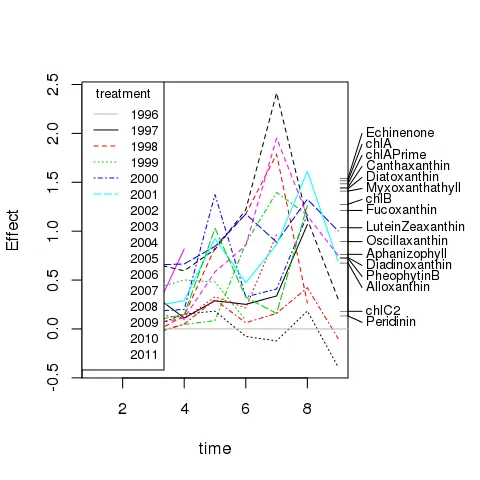
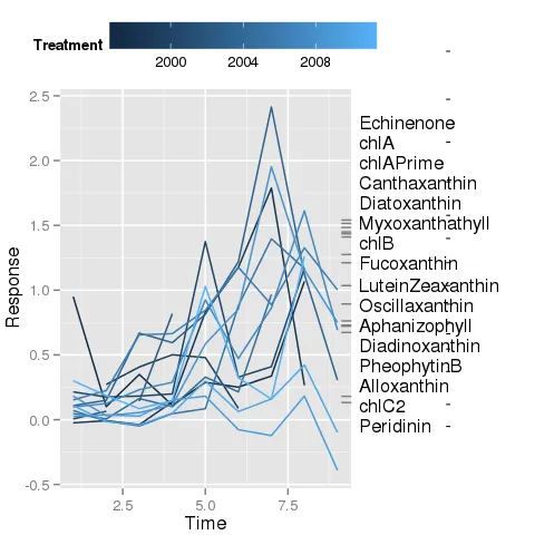
我已经成功实现了大部分内容,但目前让我困惑的是将连接右侧边际地毯图和相应标签的线段放置在何处。标签已通过anotation_custom()绘制(如下图所示),并且我使用了@baptiste的技巧关闭裁剪以允许在图形边缘绘制。
尽管我尝试了很多次,但我无法将segmentGrobs()放置在设备中所需的位置,以便它们与正确的地毯刻度和标签相连。
一个可重现的示例:
y <- data.frame(matrix(runif(30*10), ncol = 10))
names(y) <- paste0("spp", 1:10)
treat <- gl(3, 10)
time <- factor(rep(1:10, 3))

require(vegan); require(grid); require(reshape2); require(ggplot2)
mod <- prc(y, treat, time)
如果您没有安装vegan,我会在问题的末尾附上一个强化对象的dput,并提供一个fortify()方法,以便您可以运行示例并使用ggplot()进行方便的绘图。我还包括了一个相当冗长的函数myPlt(),它说明了我目前的工作情况,如果您加载了软件包并且可以创建mod,则可以对示例数据集使用它。
我已经尝试了很多选项,但现在似乎在黑暗中挣扎,无法正确放置线段。
我不是在寻找解决示例数据集绘制标签/线段的特定问题的解决方案,而是通用解决方案,可以在程序中自动放置线段和标签,因为这将构成class(mod)对象的autoplot()方法的基础。我已经解决了标签的问题,只是没有解决线段的问题。所以问题如下:
1. 当我想要放置包含从数据coord x0,y0到x1,y1运行的线的片段grob时,如何使用xmin,xmax,ymin,ymax参数? 2. 或许可以这样问,如何使用annotation_custom()在已知数据坐标x0,y0至x1,y1之间绘制位于图形区域外部的线段?
我将很高兴接收任何在图形区域中具有任何旧绘图的答案,但显示如何在图形边缘之间添加线段。
如果有更好的解决方案可用,我不会固守使用annotation_custom()。我确实想避免标签位于绘图区域中; 我认为可以通过使用annotate()并通过expand参数扩展x轴限制来实现这一点。
fortify()方法
fortify.prc <- function(model, data, scaling = 3, axis = 1,
                        ...) {
    s <- summary(model, scaling = scaling, axis = axis)
    b <- t(coef(s))
    rs <- rownames(b)
    cs <- colnames(b)
    res <- melt(b)
    names(res) <- c("Time", "Treatment", "Response")
    n <- length(s$sp)
    sampLab <- paste(res$Treatment, res$Time, sep = "-")
    res <- rbind(res, cbind(Time = rep(NA, n),
                            Treatment = rep(NA, n),
                            Response = s$sp))
    res$Score <- factor(c(rep("Sample", prod(dim(b))),
                          rep("Species", n)))
    res$Label <- c(sampLab, names(s$sp))
    res
}
dput()函数
fortify.prc(mod)的输出如下:
structure(list(Time = c(1, 2, 3, 4, 5, 6, 7, 8, 9, 10, 1, 2,
3, 4, 5, 6, 7, 8, 9, 10, NA, NA, NA, NA, NA, NA, NA, NA, NA,
NA), Treatment = c(2, 2, 2, 2, 2, 2, 2, 2, 2, 2, 3, 3, 3, 3,
3, 3, 3, 3, 3, 3, NA, NA, NA, NA, NA, NA, NA, NA, NA, NA), Response = c(0.775222658013234,
-0.0374860102875694, 0.100620532505619, 0.17475403767196, -0.736181209242918,
1.18581913245908, -0.235457236665258, -0.494834646295896, -0.22096700738071,
-0.00852429328460645, 0.102286976108412, -0.116035743892094,
0.01054849999509, 0.429857364190398, -0.29619258318138, 0.394303081010858,
-0.456401545475929, 0.391960511587087, -0.218177702859661, -0.174814586471715,
0.424769871360028, -0.0771395073436865, 0.698662414019584, 0.695676522106077,
-0.31659375422071, -0.584947748238806, -0.523065304477453, -0.19259357510277,
-0.0786143714402391, -0.313283220381509), Score = structure(c(1L,
1L, 1L, 1L, 1L, 1L, 1L, 1L, 1L, 1L, 1L, 1L, 1L, 1L, 1L, 1L, 1L,
1L, 1L, 1L, 2L, 2L, 2L, 2L, 2L, 2L, 2L, 2L, 2L, 2L), .Label = c("Sample",
"Species"), class = "factor"), Label = c("2-1", "2-2", "2-3",
"2-4", "2-5", "2-6", "2-7", "2-8", "2-9", "2-10", "3-1", "3-2",
"3-3", "3-4", "3-5", "3-6", "3-7", "3-8", "3-9", "3-10", "spp1",
"spp2", "spp3", "spp4", "spp5", "spp6", "spp7", "spp8", "spp9",
"spp10")), .Names = c("Time", "Treatment", "Response", "Score",
"Label"), row.names = c("1", "2", "3", "4", "5", "6", "7", "8",
"9", "10", "11", "12", "13", "14", "15", "16", "17", "18", "19",
"20", "spp1", "spp2", "spp3", "spp4", "spp5", "spp6", "spp7",
"spp8", "spp9", "spp10"), class = "data.frame")
我尝试过的:
myPlt <- function(x, air = 1.1) {
    ## fortify PRC model
    fx <- fortify(x)
    ## samples and species scores
    sampScr <- fx[fx$Score == "Sample", ]
    sppScr <- fx[fx$Score != "Sample", ]
    ord <- order(sppScr$Response)
    sppScr <- sppScr[ord, ]
    ## base plot
    plt <- ggplot(data = sampScr,
                  aes(x = Time, y = Response,
                      colour = Treatment, group = Treatment),
                  subset = Score == "Sample")
    plt <- plt + geom_line() + # add lines
            geom_rug(sides = "r", data = sppScr) ## add rug
    ## species labels
    sppLab <- sppScr[, "Label"]
    ## label grobs
    tg <- lapply(sppLab, textGrob, just = "left")
    ## label grob widths
    wd <- sapply(tg, function(x) convertWidth(grobWidth(x), "cm",
                                              valueOnly = TRUE))
    mwd <- max(wd) ## largest label

    ## add some space to the margin, move legend etc
    plt <- plt +
        theme(plot.margin = unit(c(0, mwd + 1, 0, 0), "cm"),
              legend.position = "top",
              legend.direction = "horizontal",
              legend.key.width = unit(0.1, "npc"))
    ## annotate locations
    ##  - Xloc = new x coord for label
    ##  - Xloc2 = location at edge of plot region where rug ticks met plot box
    Xloc <- max(fx$Time, na.rm = TRUE) +
        (2 * (0.04 * diff(range(fx$Time, na.rm = TRUE))))
    Xloc2 <- max(fx$Time, na.rm = TRUE) +
        (0.04 * diff(range(fx$Time, na.rm = TRUE)))
    ## Yloc - where to position the labels in y coordinates
    yran <- max(sampScr$Response, na.rm = TRUE) -
        min(sampScr$Response, na.rm = TRUE)
    ## This is taken from vegan:::linestack
    ## attempting to space the labels out in the y-axis direction
    ht <- 2 * (air * (sapply(sppLab,
                        function(x) convertHeight(stringHeight(x),
                                                  "npc", valueOnly = TRUE)) *
                 yran))
    n <- length(sppLab)
    pos <- numeric(n)
    mid <- (n + 1) %/% 2
    pos[mid] <- sppScr$Response[mid]
    if (n > 1) {
        for (i in (mid + 1):n) {
            pos[i] <- max(sppScr$Response[i], pos[i - 1] + ht[i])
        }
    }
    if (n > 2) {
        for (i in (mid - 1):1) {
            pos[i] <- min(sppScr$Response[i], pos[i + 1] - ht[i])
        }
    }
    ## pos now contains the y-axis locations for the labels, spread out

    ## Loop over label and add textGrob and segmentsGrob for each one
    for (i in seq_along(wd)) {
        plt <- plt + annotation_custom(tg[[i]],
                                       xmin = Xloc,
                                       xmax = Xloc,
                                       ymin = pos[i],
                                       ymax = pos[i])
        seg <- segmentsGrob(Xloc2, pos[i], Xloc, pos[i])

        ## here is problem - what to use for ymin, ymax, xmin, xmax??
        plt <- plt + annotation_custom(seg,
                                       ## xmin = Xloc2,
                                       ## xmax = Xloc,
                                       ## ymin = pos[i],
                                       ## ymax = pos[i])
                                       xmin = Xloc2,
                                       xmax = Xloc,
                                       ymin = min(pos[i], sppScr$Response[i]),
                                       ymax = max(pos[i], sppScr$Response[i]))
    }
    ## Build the plot
    p2 <- ggplot_gtable(ggplot_build(plt))
    ## turn off clipping
    p2$layout$clip[p2$layout$name=="panel"] <- "off"
    ## draw plot
    grid.draw(p2)
}
基于我在myPlt()中尝试的结果
这是我使用上面提到的myPlt()所做的进展。请注意标签上绘制的小水平刻度线 - 这些应该是上面第一个图中的倾斜线段。
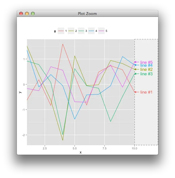
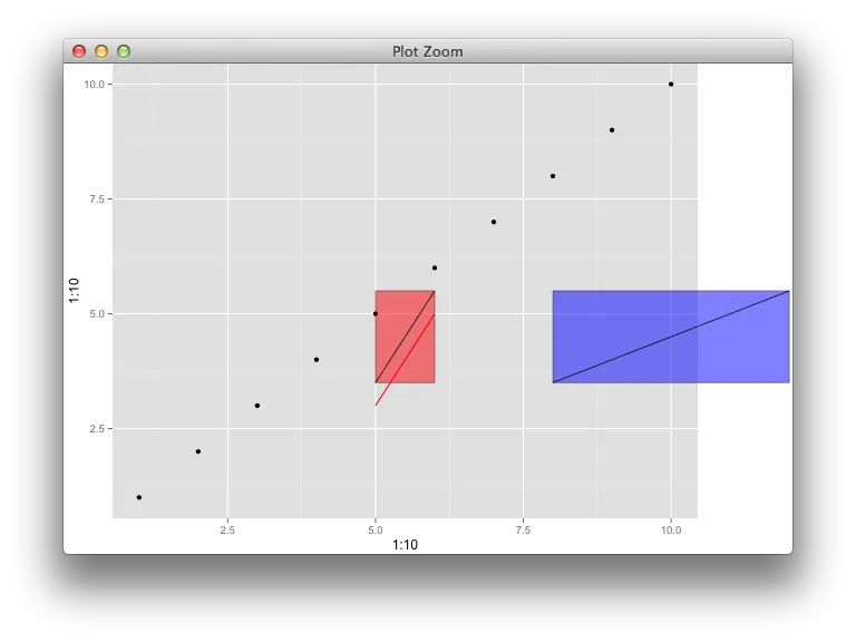
annotation_custom和关闭剪辑不是一个好的选择。你考虑过这种类型的例子吗? - baptisteannotation_custom()的工作原理。假设我想在绘图区域内放置一条连接两个已知坐标的线段。我知道如何使用annotate来实现这一点,但不知道如何使用annotation_custom()。我不明白它们之间的区别。 - Gavin Simpson