如何使用R绘制世界地图

Question

我正在开展一个项目，其中的一小部分是使用我列表中的135个国家来绘制世界地图。我还有一个列表，说明它们是否为发达国家。

我该如何在世界地图上将这些信息呈现出来，并使用不同的颜色表示它们的发展状态?

我的数据看起来像这样

Country        Code      Developed
Brazil         BRA         1
Singapore      SIN         3
France         FRA         1
Poland         POL         2

我从另一个问题中获取了下面的图片，理想情况下，它应该看起来像这样，但是要有更多的国家和3种不同的颜色。

谢谢。

- Rhedavetester

Answer 1

首先需要安装软件包：

install.packages(c("cowplot", "googleway", "ggplot2", "ggrepel", 
"ggspatial", "libwgeom", "sf", "rnaturalearth", "rnaturalearthdata")

接下来，我们将加载适用于所有地图的基本包，即ggplot2和sf。我们建议使用经典的深色背景浅色字体主题（theme_bw）适用于地图：

library("ggplot2")
theme_set(theme_bw())
library("sf")
library("rnaturalearth")
library("rnaturalearthdata")

world <- ne_countries(scale = "medium", returnclass = "sf")
class(world)

## [1] "sf"  
## [1] "data.frame"

接下来，我们可以：

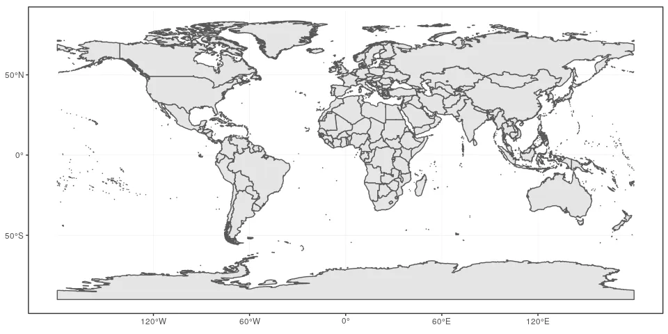
ggplot(data = world) +
    geom_sf()

结果将会是这样的：

之后，我们可以添加这个：

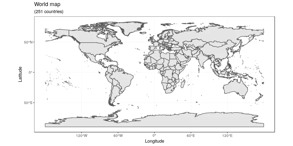
ggplot(data = world) +
    geom_sf() +
    xlab("Longitude") + ylab("Latitude") +
    ggtitle("World map", subtitle = paste0("(", length(unique(world$NAME)), " countries)"))

图表如下：

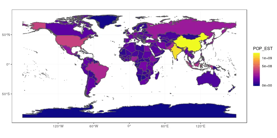
最后，如果想要一些颜色，需要这样做：

ggplot(data = world) +
    geom_sf(aes(fill = pop_est)) +
    scale_fill_viridis_c(option = "plasma", trans = "sqrt")

这个例子展示了每个国家的人口数量。在这个例子中，我们使用了“viridis”色盲友好调色板来进行颜色渐变（使用选项 =“plasma”来选择等离子体变体），使用存储在世界对象的POP_EST变量中人口数量的平方根。

您可以在此处了解更多信息:

https://r-spatial.org/r/2018/10/25/ggplot2-sf.html

https://datavizpyr.com/how-to-make-world-map-with-ggplot2-in-r/

https://slcladal.github.io/maps.html

- Danilo Mercado Oudalova

---

谢谢。这教我如何绘制地图，但没有教我如何插入我的数据。 - Rhedavetester

看链接就会知道。 :) - Danilo Mercado Oudalova

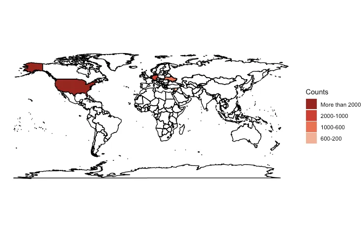
@Rhedavetester，你可以使用left_join函数将你的数据与世界上的sf数据合并。注意国家代码或名称，可以查看countrycode包来规范化你的国家名称。 - denis

Answer 2

如果你想用自己的数据来着色，你需要相应地修改world数据框：

library(rnaturalearth)
library(rnaturalearthdata)
library(ggplot2)
library(tidyverse)

world <- ne_countries(scale = "medium", returnclass = "sf")

my_countries <- c("Aruba","Afghanistan", "Morocco", "Canada")

world_modified <- world %>% 
  mutate(my_selection = ifelse(admin %in% my_countries,
                               1, NA))


ggplot(data = world_modified) +
  geom_sf(aes(fill=my_selection)) +
  theme_bw()

^{由reprex包 (v2.0.0)于2021年10月19日创建}

- MKR