我正在为某个有限大小的物理系统进行计算机模拟,之后会对无穷大进行外推(热力学极限)。一些理论认为数据应该随着系统大小呈线性缩放,因此我正在进行线性回归。
我拥有的数据存在噪声,但对于每个数据点,我可以估算误差条。例如,数据点看起来像:
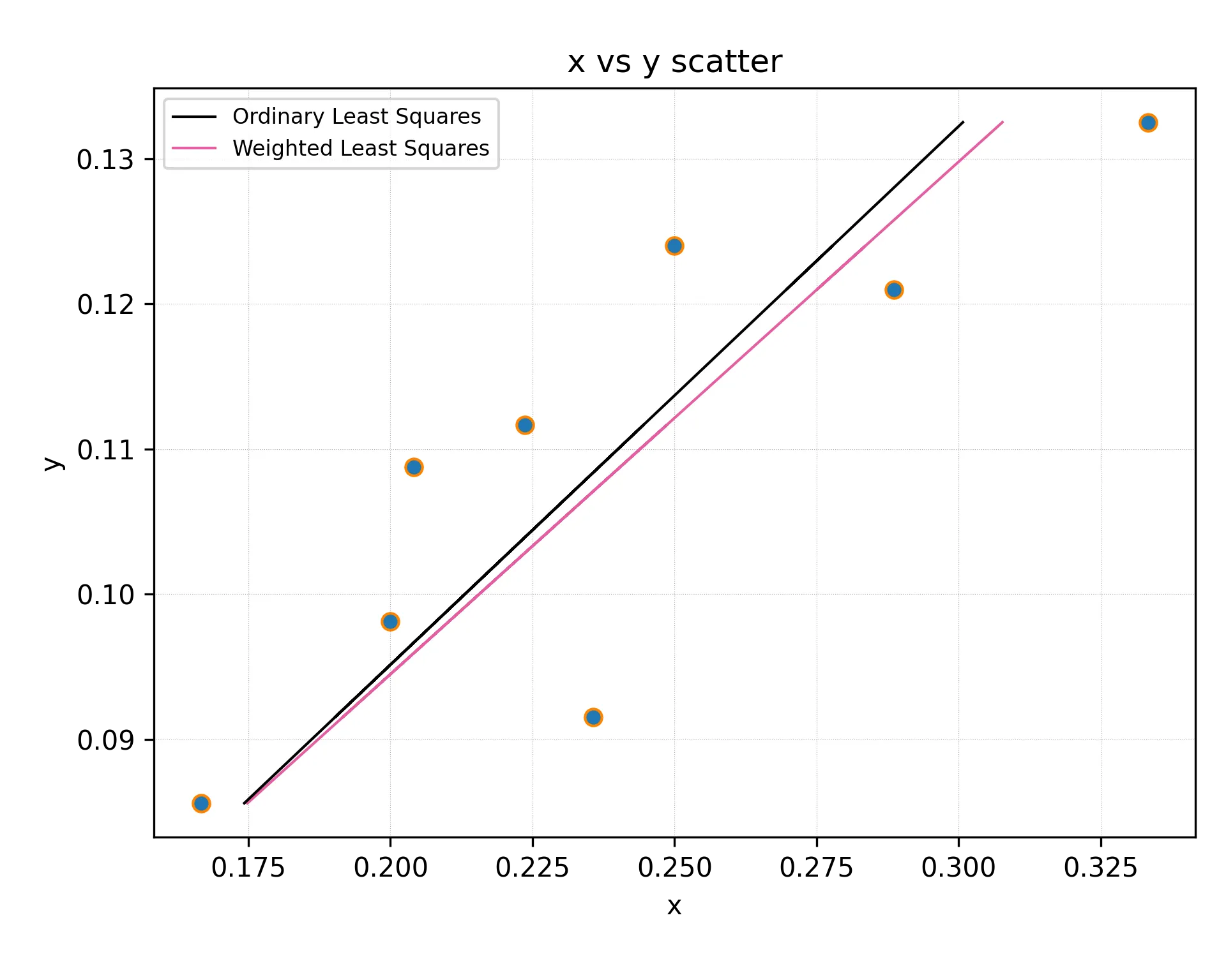
x_list = [0.3333333333333333, 0.2886751345948129, 0.25, 0.23570226039551587, 0.22360679774997896, 0.20412414523193154, 0.2, 0.16666666666666666]
y_list = [0.13250359351851854, 0.12098339583333334, 0.12398501145833334, 0.09152715, 0.11167239583333334, 0.10876248333333333, 0.09814170444444444, 0.08560799305555555]
y_err = [0.003306749165349316, 0.003818446389148108, 0.0056036878203831785, 0.0036635292592592595, 0.0037034897788415424, 0.007576672222222223, 0.002981084130692832, 0.0034913019065973983]
假设我想在Python中实现此操作。
我知道的第一种方法是:
m, c, r_value, p_value, std_err = scipy.stats.linregress(x_list, y_list)我理解这给出了结果的误差条,但是这并没有考虑到初始数据的误差条。
我知道的第二种方式是:
m, c = numpy.polynomial.polynomial.polyfit(x_list, y_list, 1, w = [1.0 / ty for ty in y_err], full=False)
但我不知道如何得到同时结合这两种方法的东西。
我真正想要的是第二种方法所做的事情,即在每个点以不同权重影响结果时使用回归。但与此同时,我想知道我的结果有多准确,也就是说,我想知道结果系数的误差条是什么。
我该怎么做?
y_err系列用作权重矩阵? - urschrei