这是一个LoG过滤的公式:
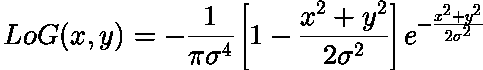
(来源:ed.ac.uk)
在使用LoG过滤的应用程序中,我看到该函数仅使用一个参数调用: sigma(σ)。 我想尝试使用该公式进行LoG过滤(之前的尝试是通过高斯滤波和带有一些滤波窗口大小的拉普拉斯滤波进行的), 但是从该公式中我无法理解滤波器的大小如何与此公式相关联,这是否意味着滤波器大小是固定的? 您能否解释如何使用它?
这是一个LoG过滤的公式:
(来源:ed.ac.uk)
在使用LoG过滤的应用程序中,我看到该函数仅使用一个参数调用: sigma(σ)。 我想尝试使用该公式进行LoG过滤(之前的尝试是通过高斯滤波和带有一些滤波窗口大小的拉普拉斯滤波进行的), 但是从该公式中我无法理解滤波器的大小如何与此公式相关联,这是否意味着滤波器大小是固定的? 您能否解释如何使用它?

private float LoG(float x, float y, float sigma)
{
    // implement formula here
    return (1 / (Math.PI * sigma*sigma*sigma*sigma)) * //etc etc - also, can't remember the code for "to the power of" off hand
}

private void GenerateTemplate(int templateSize, float sigma)
{
    // Make sure it's an odd number for convenience
    if(templateSize % 2 == 1)
    {
        // Create the data array
        float[][] template = new float[templateSize][templatesize];

        // Work out the "min and max" values. Log is centered around 0, 0
        // so, for a size 5 template (say) we want to get the values from
        // -2 to +2, ie: -2, -1, 0, +1, +2 and feed those into the formula.
        int min = Math.Ceil(-templateSize / 2) - 1;
        int max = Math.Floor(templateSize / 2) + 1;

        // We also need a count to index into the data array...
        int xCount = 0;
        int yCount = 0;

        for(int x = min; x <= max; ++x)
        {
            for(int y = min; y <= max; ++y)
            {
                // Get the LoG value for this (x,y) pair
                template[xCount][yCount] = LoG(x, y, sigma);
                ++yCount;
            }
            ++xCount;
        }
    }
}
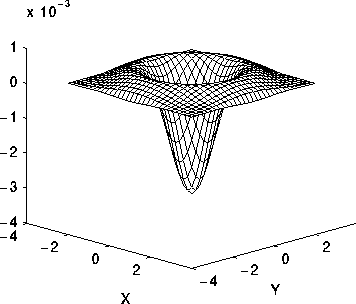
为了展示,这里有一个简单的Matlab三维彩色图,展示了拉普拉斯高斯(墨西哥帽)小波的形状。您可以更改sigma(σ)参数并观察其对图形形状的影响:
sigmaSq = 0.5 % Square of σ parameter
[x y] = meshgrid(linspace(-3,3), linspace(-3,3));
z = (-1/(pi*(sigmaSq^2))) .* (1-((x.^2+y.^2)/(2*sigmaSq))) .*exp(-(x.^2+y.^2)/(2*sigmaSq));
surf(x,y,z)
t = -5:0.01:5;
sigma = 0.5;

mexhat05 = exp(-t.*t/(2*sigma*sigma)) * 2 .*(t.*t/(sigma*sigma) - 1) / (pi^(1/4)*sqrt(3*sigma));

sigma = 1;
mexhat1 = exp(-t.*t/(2*sigma*sigma)) * 2 .*(t.*t/(sigma*sigma) - 1) / (pi^(1/4)*sqrt(3*sigma));

sigma = 2;
mexhat2 = exp(-t.*t/(2*sigma*sigma)) * 2 .*(t.*t/(sigma*sigma) - 1) / (pi^(1/4)*sqrt(3*sigma));

plot(t, mexhat05, 'r', ...
     t, mexhat1, 'b', ...
     t, mexhat2, 'g');
lb = -5; ub = 5; n = 1000;
[psi,x] = mexihat(lb,ub,n);
plot(x,psi), title('Mexican hat wavelet')
我在计算机视觉的边缘检测实现中发现这个很有用。虽然不是完全正确的答案,但希望这可以帮到你。
这似乎是一个连续的圆形滤波器,其半径为sqrt(2) * sigma。如果您想将其用于图像处理,则需要进行逼近。
这里有一个sigma = 1.4的示例:http://homepages.inf.ed.ac.uk/rbf/HIPR2/log.htm