另一个简单的解决方案使用:
代码
a=[950, 850, 750, 675, 600, 525, 460, 400, 350, 300, 250, 225, 200, 175, 150]

b = [16, 12, 9, -35, -40, -40, -40, -45, -50, -55, -60, -65, -70, -75, -80]

c=[32.0, 22.2, 12.399999999999999, 2.599999999999998, -7.200000000000003, -17.0, -26.800000000000004, -36.60000000000001, -46.400000000000006, -56.2, -66.0, -75.80000000000001, -85.60000000000001, -95.4, -105.20000000000002]
from sklearn.linear_model import LinearRegression
from scipy.optimize import minimize
import numpy as np
reg_a = LinearRegression().fit(np.arange(len(a)).reshape(-1,1), a)
reg_b = LinearRegression().fit(np.arange(len(b)).reshape(-1,1), b)
reg_c = LinearRegression().fit(np.arange(len(c)).reshape(-1,1), c)
funA = lambda x: reg_a.predict(x.reshape(-1,1))
funB = lambda x: reg_b.predict(x.reshape(-1,1))
funC = lambda x: reg_c.predict(x.reshape(-1,1))
opt_crossing = lambda x: (funB(x) - funC(x))**2
x0 = 1
res = minimize(opt_crossing, x0, method='SLSQP', tol=1e-6)
print(res)
print('Solution: ', funA(res.x))
import matplotlib.pyplot as plt
x = np.linspace(0, 15, 100)
a_ = reg_a.predict(x.reshape(-1,1))
b_ = reg_b.predict(x.reshape(-1,1))
c_ = reg_c.predict(x.reshape(-1,1))
plt.plot(x, a_, color='blue')
plt.plot(x, b_, color='green')
plt.plot(x, c_, color='cyan')
plt.scatter(np.arange(15), a, color='blue')
plt.scatter(np.arange(15), b, color='green')
plt.scatter(np.arange(15), c, color='cyan')
plt.axvline(res.x, color='red', linestyle='solid')
plt.axhline(funA(res.x), color='red', linestyle='solid')
plt.show()
输出
fun: array([  7.17320622e-15])
jac: array([ -3.99479864e-07,   0.00000000e+00])
message: 'Optimization terminated successfully.'
nfev: 8
nit: 2
njev: 2
status: 0
success: True
  x: array([ 8.37754008])
Solution:  [ 379.55151658]
绘图
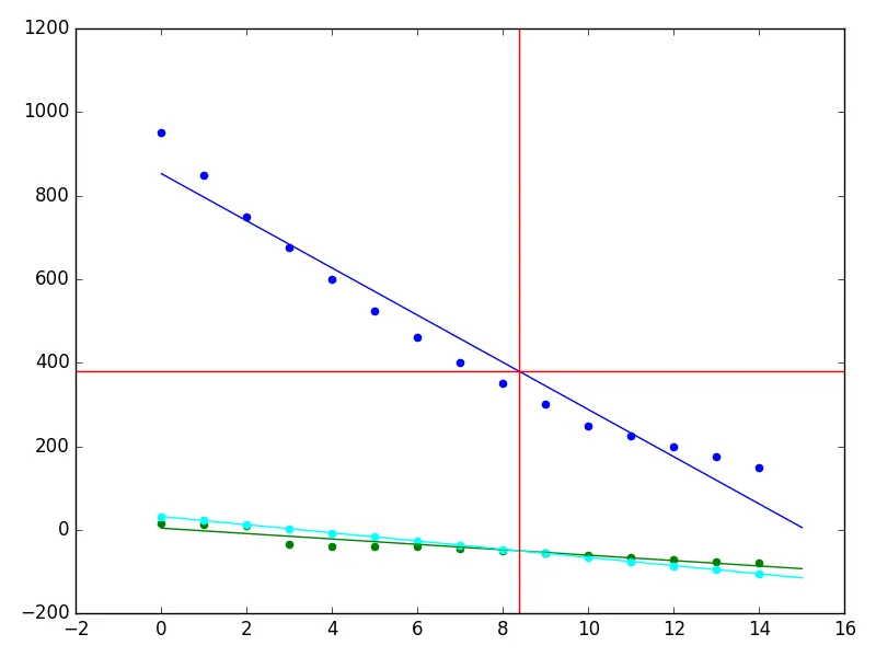
a、b和c的示例吗? - Christian Ternus