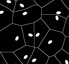
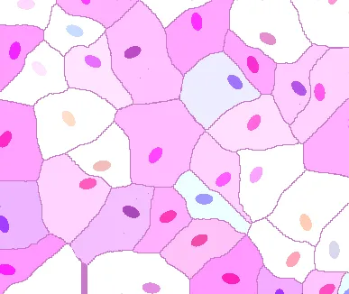
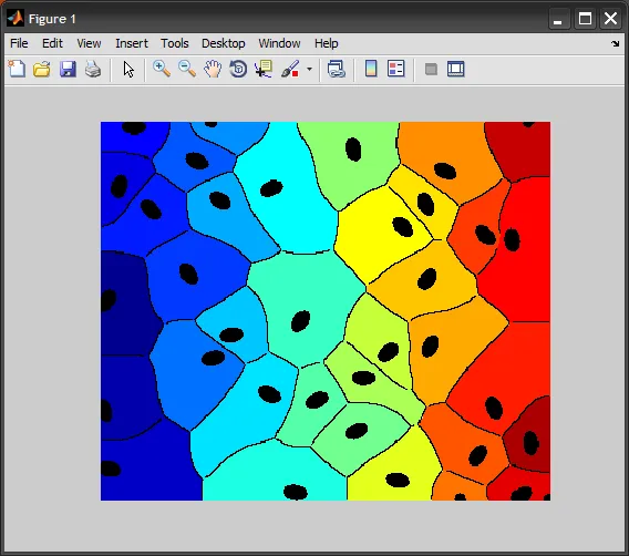
我手头有一张图像(png格式),椭圆形的边界线(代表细胞核)是直线,不太实用。我该如何从图像中提取这些线并使其弯曲,前提是它们仍然围绕着细胞核。
以下是该图像:
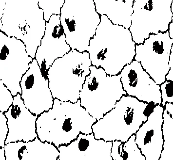
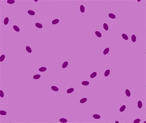
 弯曲后:
弯曲后:
 编辑:如何将答案2中的“膨胀和过滤”部分翻译成Matlab语言?我想不出来。
以下是该图像:
弯曲后:
编辑:如何将答案2中的“膨胀和过滤”部分翻译成Matlab语言?我想不出来。
弯曲后:
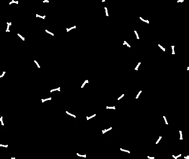
编辑:如何将答案2中的“膨胀和过滤”部分翻译成Matlab语言?我想不出来。i3是没有线条的输入图像):ColorCombine[{Image[
WatershedComponents[
DistanceTransform[Binarize@i3,
DistanceFunction -> ManhattanDistance] ]], i3, i3}]
编辑
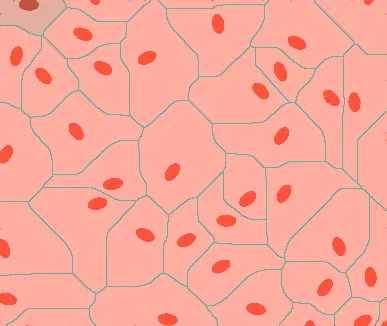
我正在使用另一种算法(初步结果)。您觉得如何?
好的,这里有一种方法涉及到几个随机化步骤,能够获得“自然”非对称外观。
我发布了实际的Mathematica代码,以防万一有人需要将其翻译为Matlab。
(* A preparatory step: get your image and clean it*)
i = Import@"http://i.stack.imgur.com/YENhB.png";
i1 = Image@Replace[ImageData[i], {0., 0., 0.} -> {1, 1, 1}, {2}];
i2 = ImageSubtract[i1, i];
i3 = Inpaint[i, i2]
(*Now reduce to a skeleton to get a somewhat random starting point.
The actual algorithm for this dilation does not matter, as far as we
get a random area slightly larger than the original elipses *)
id = Dilation[SkeletonTransform[
             Dilation[SkeletonTransform@ColorNegate@Binarize@i3, 3]], 1]
(*Now the real random dilation loop*)
(*Init vars*)
p = Array[1 &, 70]; j = 1;
(*Store in w an image with a different color for each cluster, so we
can find edges between them*)
w = (w1 =
      WatershedComponents[
       GradientFilter[Binarize[id, .1], 1]]) /. {4 -> 0} // Colorize;
(*and loop ...*)
For[i = 1, i < 70, i++,
 (*Select edges in w and dilate them with a random 3x3 kernel*)
 ed = Dilation[EdgeDetect[w, 1], RandomInteger[{0, 1}, {3, 3}]];
 (*The following is the core*)
 p[[j++]] = w =
   ImageFilter[  (* We apply a filter to the edges*)
    (Switch[
          Length[#1],  (*Count the colors in a 3x3 neighborhood of each pixel*)
          0, {{{0, 0, 0}, 0}},          (*If no colors, return bkg*)
          1, #1,                        (*If one color, return it*)
          _, {{{0, 0, 0}, 0}}])[[1, 1]] (*If more than one color, return bkg*)&@
      Cases[Tally[Flatten[#1, 1]],
       Except[{{0.`, 0.`, 0.`}, _}]] & (*But Don't count bkg pixels*),
    w, 1,
    Masking -> ed,       (*apply only to edges*)
    Interleaving -> True (*apply to all color chanels at once*)]
 ]
结果是:
编辑
对于以Mathematica为导向的读者来说,最后一个循环的功能代码可能更容易(且更短):
NestList[
 ImageFilter[
   If[Length[#1] ==  1, #1[[1, 1]], {0, 0, 0}] &@
     Cases[Tally[Flatten[#1, 1]], Except[{0.` {1, 1, 1}, _}]] & , #, 1,
   Masking      -> Dilation[EdgeDetect[#, 1], RandomInteger[{0, 1}, {3, 3}]],
   Interleaving -> True ] &,
 WatershedComponents@GradientFilter[Binarize[id,.1],1]/.{4-> 0}//Colorize,
5]
这是我想到的翻译,它不是@belisarius代码的直接翻译,但应该足够接近。
%# read image (indexed image)
[I,map] = imread('http://i.stack.imgur.com/YENhB.png');

%# extract the blobs (binary image)
BW = (I==1);

%# skeletonization + dilation
BW = bwmorph(BW, 'skel', Inf);
BW = imdilate(BW, strel('square',2*1+1));

%# connected components
L = bwlabel(BW);
imshow(label2rgb(L))

%# filter 15x15 neighborhood
for i=1:13
    L = nlfilter(L, [15 15], @myFilterFunc);
    imshow( label2rgb(L) )
end

%# result
L(I==1) = 0;                %# put blobs back
L(edge(L,'canny')) = 0;     %# edges
imshow( label2rgb(L,@jet,[0 0 0]) )
function p = myFilterFunc(x)
    if range(x(:)) == 0
        p = x(1);                %# if one color, return it
    else
        p = mode(x(x~=0));       %# else, return the most frequent color
    end
end
结果:
以下是该过程的动画: