如何将直方图归一化,使得概率密度函数下的面积等于1?
7个回答
123
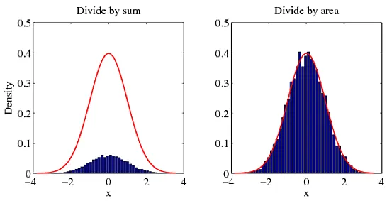
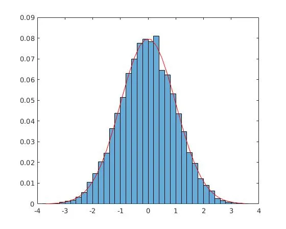
我的回答与你之前的问题中的回答相同。对于概率密度函数,整个空间上的积分为1。除以总和不会给出正确的密度。要获得正确的密度,必须除以面积。为了说明我的观点,请尝试以下示例。
[f, x] = hist(randn(10000, 1), 50); % Create histogram from a normal distribution.
g = 1 / sqrt(2 * pi) * exp(-0.5 * x .^ 2); % pdf of the normal distribution

% METHOD 1: DIVIDE BY SUM
figure(1)
bar(x, f / sum(f)); hold on
plot(x, g, 'r'); hold off

% METHOD 2: DIVIDE BY AREA
figure(2)
bar(x, f / trapz(x, f)); hold on
plot(x, g, 'r'); hold off
你可以亲自查看哪种方法与正确答案(红色曲线)相符。
将直方图归一化的另一种方法(比方法2更直接)是通过除以sum(f * dx)来表达概率密度函数的积分。
% METHOD 3: DIVIDE BY AREA USING sum()
figure(3)
dx = diff(x(1:2))
bar(x, f / sum(f * dx)); hold on
plot(x, g, 'r'); hold off
- user616736
5
2“除以面积图形”的总和不等于1。我看到至少有10个条形图点大于0.3。0.3 * 10 = 3.0。难道把f除以样本数量(在这种情况下为10000)不是更简单的解决方案吗? - Rich
9@Rich,这些条比1更细,所以你的计算是错误的。考虑曲线下三角形从(-2,0)到(0,0.4)到(2,0)来估算面积。这个三角形的面积为0.540.4 = 0.8 < 1.0。 - neingeist
2要使和等于1,需要将新的箱子总和乘以箱子宽度。 - alperovich
@abcd:但是这篇文章说,我们可以通过总和进行归一化处理:http://www.itl.nist.gov/div898/handbook/eda/section3/histogra.htm - kmario23
1如何使用histcounts而不是hist来完成这个任务? - Pedro77
24
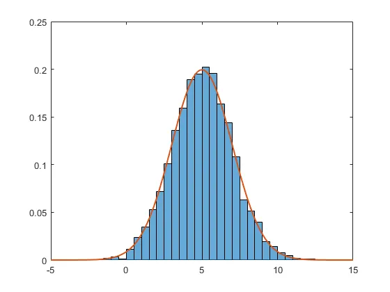
自2014b版本以来,Matlab在
histogram函数中原生嵌入了这些标准化例程(请参见帮助文件,了解此函数提供的6个例程)。以下是使用PDF标准化的示例(所有条形桶的总和为1)。data = 2*randn(5000,1) + 5; % generate normal random (m=5, std=2)
h = histogram(data,'Normalization','pdf') % PDF normalization
相应的PDF文档是
Nbins = h.NumBins;
edges = h.BinEdges;
x = zeros(1,Nbins);
for counter=1:Nbins
    midPointShift = abs(edges(counter)-edges(counter+1))/2;
    x(counter) = edges(counter)+midPointShift;
end

mu = mean(data);
sigma = std(data);

f = exp(-(x-mu).^2./(2*sigma^2))./(sigma*sqrt(2*pi));
两者结合在一起
hold on;
plot(x,f,'LineWidth',1.5)
这可能是由于实际问题和被接受的答案的成功而带来的改进!
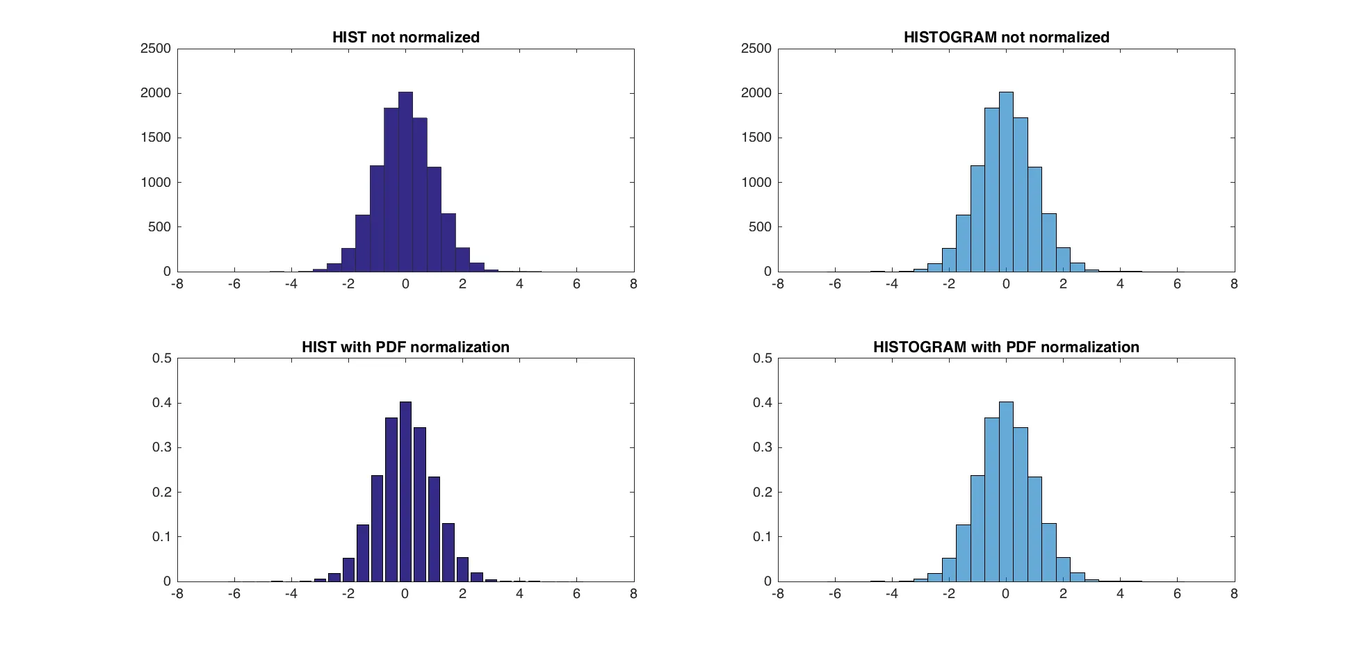
编辑 - 现在不建议使用hist和histc,应该使用histogram。请注意,使用这个新函数创建6种方式中的任何一种都不会产生hist和histc生成的bins。有一个Matlab脚本可以更新以前的代码,以适应调用histogram的方式(使用bin边缘而不是bin中心-link)。通过这样做,可以比较@abcd(trapz和sum)和Matlab(pdf)的pdf归一化方法。
3种pdf归一化方法的结果几乎相同(在eps范围内)。
测试:
A = randn(10000,1);
centers = -6:0.5:6;
d = diff(centers)/2;
edges = [centers(1)-d(1), centers(1:end-1)+d, centers(end)+d(end)];
edges(2:end) = edges(2:end)+eps(edges(2:end));

figure;
subplot(2,2,1);
hist(A,centers);
title('HIST not normalized');

subplot(2,2,2);
h = histogram(A,edges);
title('HISTOGRAM not normalized');

subplot(2,2,3)
[counts, centers] = hist(A,centers); %get the count with hist
bar(centers,counts/trapz(centers,counts))
title('HIST with PDF normalization');


subplot(2,2,4)
h = histogram(A,edges,'Normalization','pdf')
title('HISTOGRAM with PDF normalization');

dx = diff(centers(1:2))
normalization_difference_trapz = abs(counts/trapz(centers,counts) - h.Values);
normalization_difference_sum = abs(counts/sum(counts*dx) - h.Values);

max(normalization_difference_trapz)
max(normalization_difference_sum)
- marsei
1
PDF下的面积不应该是直方图中的1,这在概率论中是不可能的。请参考stackoverflow.com/a/38813376/54964中的答案进行一些更正。为了使pdf下的面积为1,您应该将归一化设置为“probability”,而不是“pdf”。 - Léo Léopold Hertz 준영
5
[f,x]=hist(data)
每个矩形的面积为高度和宽度的乘积。由于MATLAB会选择等间距的点作为矩形的位置,因此其宽度为:
delta_x = x(2) - x(1)
现在,如果我们将所有单独的条形图相加,总面积将为:
A=sum(f)*delta_x
因此,正确缩放的图表可通过以下方式获得:
bar(x, f/sum(f)/(x(2)-x(1)))
- Moppi
3
abcd的PDF面积不是1,正如许多评论所指出的那样,这是不可能的。在这里做出了许多答案的假设
- 假设连续边缘之间的距离是恒定的。
pdf下的概率应为1。归一化应该作为probability进行,而不是作为pdf进行,在histogram()和hist()中进行。
图1 hist()方法的输出,图2 histogram()方法的输出
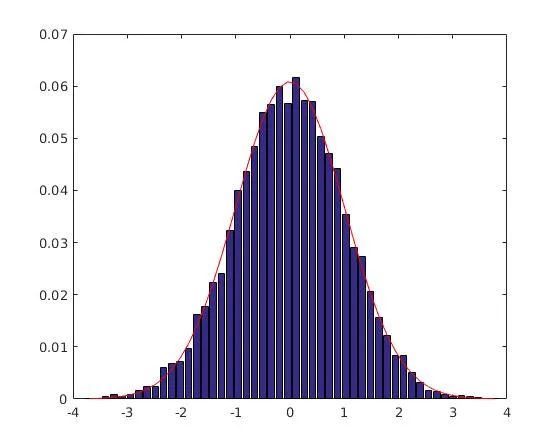
两种方法之间的最大振幅不同,这表明hist()的方法存在一些错误,因为histogram()的方法使用了标准归一化。我认为这里hist()方法的错误部分在于归一化只是部分地作为pdf,而不完全作为probability。
使用hist()的代码[已弃用]
一些说明
- 首先检查:
sum(f)/N如果手动设置了Nbins,则会给出1。 pdf需要图形g中的bin的宽度(dx)
代码
%https://dev59.com/0m435IYBdhLWcg3wmxTz#5321546
N=10000;
Nbins=50;
[f,x]=hist(randn(N,1),Nbins); % create histogram from ND

%METHOD 4: Count Densities, not Sums!
figure(3)
dx=diff(x(1:2)); % width of bin
g=1/sqrt(2*pi)*exp(-0.5*x.^2) .* dx; % pdf of ND with dx
% 1.0000
bar(x, f/sum(f));hold on
plot(x,g,'r');hold off
输出结果见图1。
使用histogram()函数的代码
一些注意事项
- 第一步检查:a)如果将
Normalization设置为概率,则sum(f)应为1;b)如果手动设置Nbins而不进行标准化,则sum(f)/N应为1。 pdf需要图形g中每个条柱的宽度(即dx)。
代码:
%%METHOD 5: with histogram()
% http://stackoverflow.com/a/38809232/54964
N=10000;

figure(4);
h = histogram(randn(N,1), 'Normalization', 'probability') % hist() deprecated!
Nbins=h.NumBins;
edges=h.BinEdges;
x=zeros(1,Nbins);
f=h.Values;
for counter=1:Nbins
    midPointShift=abs(edges(counter)-edges(counter+1))/2; % same constant for all
    x(counter)=edges(counter)+midPointShift;
end
dx=diff(x(1:2)); % constast for all
g=1/sqrt(2*pi)*exp(-0.5*x.^2) .* dx; % pdf of ND
% Use if Nbins manually set
%new_area=sum(f)/N % diff of consecutive edges constant
% Use if histogarm() Normalization probability
new_area=sum(f)
% 1.0000
% No bar() needed here with histogram() Normalization probability
hold on;
plot(x,g,'r');hold off
图2的输出和预期输出相符:面积为1.0000。
Matlab版本:2016a
系统:Linux Ubuntu 16.04 64位
Linux内核版本:4.6
- Léo Léopold Hertz 준영
6
我和楼主有同样的问题,让我困惑的是你所说的与MATLAB文档完全相反。请查看https://www.mathworks.com/help/matlab/ref/histogram.html#input_argument_namevalue_Normalization它明确表示要使用“pdf”使条形区域总和为1而不是“probability”。此外,您正在使用
sum(f),其中f = h.Values以显示面积为1。 h.Values对应于bin高度,因此根据“probability”规范的定义,这将总和为1,但这与条形区域不同。 - ITA1使用histogram()编写代码:如果您将randn(N,1)乘以某个常数,那么红线将不再与数据匹配。 - Pedro77
我正在使用@marsei的答案。当我的直方图不是“非常”正常时,我会使用拟合的样条曲线到h.Value。 - Pedro77
1对于非正常情况: [曲线, 拟合优度, 输出] = fit(x(:),h.Values(:),'smoothingspline','SmoothingParam',0.9999999); lPlot = plot(x(:),曲线(x));。对于正常情况,请参考@marsei的答案。 - Pedro77
@Pedro77,您能否直接编辑此答案以显示您将进行更改的位置? - Léo Léopold Hertz 준영
1
对于某些分布,比如柯西分布,我发现trapz函数会高估面积,因此概率密度函数会根据您选择的箱数而改变。在这种情况下,我会
[N,h]=hist(q_f./theta,30000); % there Is a large range but most of the bins will be empty
plot(h,N/(sum(N)*mean(diff(h))),'+r')
- user1240280
1
嗨!数量 mean(diff(h)) 是否应该是箱子的宽度? - Daddy Kropotkin
网页内容由stack overflow 提供, 点击上面的可以查看英文原文,
原文链接
原文链接