我有一组包含加速度数据的时间序列,希望将其积分成速度和位移时间序列。这可以使用FFT完成,但是在Matlab和Python中使用两种方法得到了不同的结果。
Matlab代码:
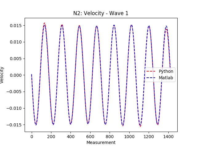
这两个代码通常应该给出完全相同的结果,但是当我进行比较绘图时,得到了以下结果。
加速度转速度。
我还有第二个Python版本,其中我尝试包含Matlab代码中的滤波器。这也会给出不同的结果,就像Python中没有滤波器的结果一样。
这仍然与Matlab代码略有不同。有建议吗?
Matlab代码:
nsamples = length(acc(:,1));
domega = 2*pi/(dt*nsamples);
acchat = fft(acc);

% Make frequency array:
Omega = zeros(nsamples,1);

% Create Omega:
if even(nsamples)
   nh = nsamples/2;
   Omega(1:nh+1) = domega*(0:nh);
   Omega(nh+2:nsamples) = domega*(-nh+1:-1);
else
   nh = (nsamples-1)/2;
   Omega(1:nh+1) = domega*(0:nh);
   Omega(nh+2:nsamples) = domega*(-nh:-1);
end

% High-pass filter:
n_low=floor(2*pi*f_low/domega);
acchat(1:n_low)=0;
acchat(nsamples-n_low+1:nsamples)=0;

% Multiply by omega^2:
acchat(2:nsamples) = -acchat(2:nsamples) ./ Omega(2:nsamples).^2;

% Inverse Fourier transform:
pos = real(ifft(acchat));

% --- End of function ---
Python 代码:
import numpy as np


def acc2velpos(acc, dt):

    n = len(acc)

    freq = np.fft.fftfreq(n, d=dt)
    omegas = 2 * np.pi * freq
    omegas = omegas[1:]

    # Fast Fourier Transform of Acceleration
    accfft = np.array(np.fft.fft(acc, axis=0))

    # Integrating the Fast Fourier Transform
    velfft = -accfft[1:] / (omegas * 1j)
    posfft = accfft[1:] / ((omegas * 1j) ** 2)

    velfft = np.array([0] + list(velfft))
    posfft = np.array([0] + list(posfft))

    # Inverse Fast Fourier Transform back to time domain
    vel = np.real(np.fft.ifft(velfft, axis=0))
    pos = np.real(np.fft.ifft(posfft, axis=0))

    return vel, pos
这两个代码通常应该给出完全相同的结果,但是当我进行比较绘图时,得到了以下结果。
加速度转速度。
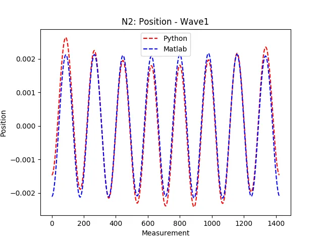
我还有第二个Python版本,其中我尝试包含Matlab代码中的滤波器。这也会给出不同的结果,就像Python中没有滤波器的结果一样。
def acc2vel2(acc, dt, flow):

    nsamples = len(acc)
    domega = (2*np.pi) / (dt*nsamples)
    acchat = np.fft.fft(acc)

    # Make Freq. Array
    Omega = np.zeros(nsamples)

    # Create Omega:
    if nsamples % 2 == 0:
        nh = int(nsamples/2)
        Omega[:nh] = domega * np.array(range(0, nh))
        Omega[nh:] = domega * np.array(range(-nh-1, -1))

    else:
        nh = int((nsamples - 1)/2)
        Omega[:nh] = domega * np.array(range(0, nh))
        Omega[nh:] = domega * np.array(range(-nh-2, -1))

    # High-pass filter
    n_low = int(np.floor((2*np.pi*flow)/domega))
    acchat[:n_low - 1] = 0
    acchat[nsamples - n_low:] = 0

    # Divide by omega
    acchat[1:] = -acchat[1:] / Omega[1:]

    # Inverse FFT
    vel = np.imag(np.fft.ifft(acchat))

return vel
这仍然与Matlab代码略有不同。有建议吗?