使用ggplot2重现drc::plot.drc

Question

使用ggplot2重现drc::plot.drc

4

我希望使用ggplot2画出以下drc::plot.drc的图形。

df1 <-
      structure(list(TempV = structure(c(1L, 1L, 1L, 1L, 1L, 1L, 1L, 
    1L, 1L, 1L, 5L, 5L, 5L, 5L, 5L, 5L, 5L, 5L, 5L, 5L, 3L, 3L, 3L, 
    3L, 3L, 3L, 3L, 3L, 3L, 3L, 7L, 7L, 7L, 7L, 7L, 7L, 7L, 7L, 7L, 
    7L, 9L, 9L, 9L, 9L, 9L, 9L, 9L, 9L, 9L, 9L, 13L, 13L, 13L, 13L, 
    13L, 13L, 13L, 13L, 13L, 13L, 11L, 11L, 11L, 11L, 11L, 11L, 11L, 
    11L, 11L, 11L, 2L, 2L, 2L, 2L, 2L, 2L, 2L, 2L, 2L, 2L, 6L, 6L, 
    6L, 6L, 6L, 6L, 6L, 6L, 6L, 6L, 4L, 4L, 4L, 4L, 4L, 4L, 4L, 4L, 
    4L, 4L, 8L, 8L, 8L, 8L, 8L, 8L, 8L, 8L, 8L, 8L, 10L, 10L, 10L, 
    10L, 10L, 10L, 10L, 10L, 10L, 10L, 14L, 14L, 14L, 14L, 14L, 14L, 
    14L, 14L, 14L, 14L, 12L, 12L, 12L, 12L, 12L, 12L, 12L, 12L, 12L, 
    12L), .Label = c("22.46FH-142", "27.59FH-142", "26.41FH-142", 
    "29.71FH-142", "31.66FH-142", "34.11FH-142", "33.22FH-142", "22.46FH-942", 
    "27.59FH-942", "26.41FH-942", "29.71FH-942", "31.66FH-942", "34.11FH-942", 
    "33.22FH-942"), class = "factor"), Start = c(0L, 24L, 48L, 72L, 
    96L, 120L, 144L, 168L, 192L, 216L, 0L, 24L, 48L, 72L, 96L, 120L, 
    144L, 168L, 192L, 216L, 0L, 24L, 48L, 72L, 96L, 120L, 144L, 168L, 
    192L, 216L, 0L, 24L, 48L, 72L, 96L, 120L, 144L, 168L, 192L, 216L, 
    0L, 24L, 48L, 72L, 96L, 120L, 144L, 168L, 192L, 216L, 0L, 24L, 
    48L, 72L, 96L, 120L, 144L, 168L, 192L, 216L, 0L, 24L, 48L, 72L, 
    96L, 120L, 144L, 168L, 192L, 216L, 0L, 24L, 48L, 72L, 96L, 120L, 
    144L, 168L, 192L, 216L, 0L, 24L, 48L, 72L, 96L, 120L, 144L, 168L, 
    192L, 216L, 0L, 24L, 48L, 72L, 96L, 120L, 144L, 168L, 192L, 216L, 
    0L, 24L, 48L, 72L, 96L, 120L, 144L, 168L, 192L, 216L, 0L, 24L, 
    48L, 72L, 96L, 120L, 144L, 168L, 192L, 216L, 0L, 24L, 48L, 72L, 
    96L, 120L, 144L, 168L, 192L, 216L, 0L, 24L, 48L, 72L, 96L, 120L, 
    144L, 168L, 192L, 216L), End = c(24, 48, 72, 96, 120, 144, 168, 
    192, 216, Inf, 24, 48, 72, 96, 120, 144, 168, 192, 216, Inf, 
    24, 48, 72, 96, 120, 144, 168, 192, 216, Inf, 24, 48, 72, 96, 
    120, 144, 168, 192, 216, Inf, 24, 48, 72, 96, 120, 144, 168, 
    192, 216, Inf, 24, 48, 72, 96, 120, 144, 168, 192, 216, Inf, 
    24, 48, 72, 96, 120, 144, 168, 192, 216, Inf, 24, 48, 72, 96, 
    120, 144, 168, 192, 216, Inf, 24, 48, 72, 96, 120, 144, 168, 
    192, 216, Inf, 24, 48, 72, 96, 120, 144, 168, 192, 216, Inf, 
    24, 48, 72, 96, 120, 144, 168, 192, 216, Inf, 24, 48, 72, 96, 
    120, 144, 168, 192, 216, Inf, 24, 48, 72, 96, 120, 144, 168, 
    192, 216, Inf, 24, 48, 72, 96, 120, 144, 168, 192, 216, Inf), 
        Germinated = c(0L, 0L, 0L, 0L, 3L, 67L, 46L, 12L, 101L, 221L, 
        0L, 0L, 0L, 0L, 57L, 50L, 44L, 31L, 32L, 236L, 0L, 0L, 0L, 
        31L, 68L, 50L, 31L, 34L, 29L, 207L, 0L, 0L, 8L, 30L, 31L, 
        55L, 27L, 22L, 4L, 273L, 0L, 0L, 46L, 64L, 16L, 8L, 15L, 
        15L, 20L, 266L, 0L, 0L, 0L, 0L, 4L, 13L, 63L, 51L, 147L, 
        172L, 0L, 0L, 4L, 26L, 92L, 31L, 91L, 14L, 7L, 185L, 0L, 
        0L, 0L, 0L, 0L, 32L, 59L, 36L, 50L, 273L, 0L, 0L, 0L, 4L, 
        13L, 32L, 42L, 52L, 42L, 265L, 0L, 0L, 0L, 6L, 22L, 40L, 
        57L, 44L, 73L, 208L, 0L, 1L, 2L, 24L, 55L, 41L, 68L, 24L, 
        33L, 202L, 0L, 0L, 18L, 31L, 26L, 30L, 61L, 25L, 58L, 201L, 
        0L, 0L, 36L, 54L, 33L, 55L, 12L, 27L, 55L, 178L, 0L, 0L, 
        6L, 28L, 26L, 31L, 53L, 48L, 33L, 225L)), .Names = c("TempV", 
    "Start", "End", "Germinated"), row.names = c(NA, -140L), class = "data.frame")

library(data.table)

dt1 <- data.table(df1)

library(drc)

dt1fm1 <- 
  drm(
        formula   = Germinated ~ Start + End
      , curveid   = TempV
  #   , pmodels   = 
  #   , weights   = 
      , data      = dt1
  #   , subset    = 
      , fct       = LL.2()
      , type      = "event"
      , bcVal     = NULL
      , bcAdd     = 0
  #   , start     =
      , na.action = na.fail
      , robust    = "mean"
      , logDose   = NULL
      , control   = drmc(
                            constr      = FALSE
                            , errorm      = TRUE
                            , maxIt       = 1500
                            , method      = "BFGS"
                            , noMessage   = FALSE
                            , relTol      = 1e-07
                            , rmNA        = FALSE
                            , useD        = FALSE
                            , trace       = FALSE
                            , otrace      = FALSE
                            , warnVal     = -1
                            , dscaleThres = 1e-15
                            , rscaleThres = 1e-15
                            )
      , lowerl    = NULL
      , upperl    = NULL
      , separate  = FALSE
      , pshifts   = NULL 
      )



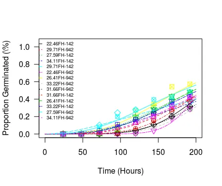
## ----dt1fm1Plot1----
plot(
        x      = dt1fm1
    , xlab     = "Time (Hours)"
    , ylab     = "Proportion Germinated (\\%)"    
  # , ylab     = "Proportion Germinated (%)"    
    , add      = FALSE
    , level    = NULL
    , type     = "average" # c("average", "all", "bars", "none", "obs", "confidence")
    , broken   = FALSE
  # , bp
    , bcontrol = NULL
    , conName  = NULL
    , axes     = TRUE
    , gridsize = 100
    , log      = ""
  # , xtsty
    , xttrim   = TRUE
    , xt       = NULL
    , xtField    = NULL
    , xField     = "Time (Hours)"
    , xlim     = c(0, 200)
    , yt       = NULL
    , ytField    = NULL
    , yField     = "Proportion Germinated"
    , ylim     = c(0, 1.05)
    , lwd      = 1
    , cex      = 1.2
    , cex.axis = 1
    , col      = TRUE
  # , lty
  # , pch
    , legend     = TRUE
  # , legendText  
    , legendPos  = c(40, 1.1)
    , cex.legend = 0.6
    , normal     = FALSE
    , normRef    = 1
    , confidence.level = 0.95
    )


## ----dt1fm1Plot2----
dt1fm1Means1 <- dt1[, .(Germinated=mean(Germinated)/450), by=.(TempV, Start, End)]
dt1fm1Means2 <- dt1fm1Means1[, .(Start=Start, End=End, Cum_Germinated=cumsum(Germinated)), by=.(TempV)]
dt1fm1Means  <- data.table(dt1fm1Means2[End!=Inf], Pred=predict(object=dt1fm1))

dt1fm1Plot2 <- 
       ggplot(data= dt1fm1Means, mapping=aes(x=End, y=Cum_Germinated, group=TempV, color=TempV, shape=TempV)) + 
        geom_point() +
        geom_line(aes(y = Pred)) +
        scale_shape_manual(values=seq(0, 13)) +
        labs(x = "Time (Hours)", y = "Proportion Germinated", shape="Temp", color="Temp") +
        theme_bw() +
        scale_x_continuous(expand = c(0, 0), breaks = c(0, unique(dt1fm1Means$End))) +
        scale_y_continuous(expand = c(0, 0), labels = function(x) paste0(100*x,"\\%")) +
      # scale_y_continuous(expand = c(0, 0), labels = percent) +
        expand_limits(x = c(0, max(dt1fm1Means$End)+20), y = c(0, max(dt1fm1Means$Pred)+0.1)) +
        theme(axis.title.x = element_text(size = 12, hjust = 0.54, vjust = 0),
              axis.title.y = element_text(size = 12, angle = 90,  vjust = 0.25))
print(dt1fm1Plot2)

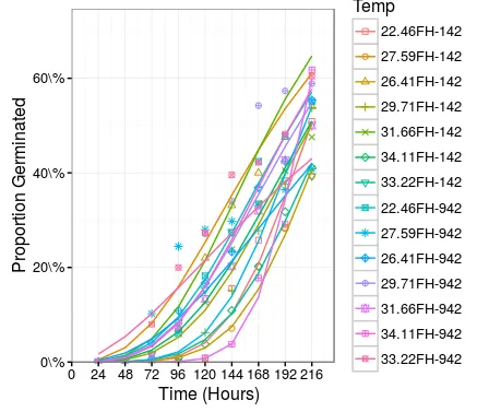
问题

ggplot2 输出中存在一些差异。这些差异是由于 predict 函数给出的输出与数据中给定的水平不同。

编辑后

实际上，drm 函数改变了 TempV 的水平顺序，这在 summary(dt1fm1) 输出和 drc::plot.drc 输出的图表中很清楚。

- MYaseen208

我之前有一个类似的问题：https://dev59.com/TJbfa4cB1Zd3GeqPsFQM#37043751。简而言之，我能够使用stat_smooth函数直接绘制drm模型，但由于某种原因，这种行为在我测试的所有机器上都没有重复出现。另一种选择是将预测值添加到数据集中并绘制这些值。 - biomiha

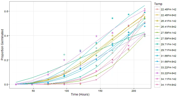
biomiha: 在@dww的帮助下，我已经弄清楚了如何使用ggplot2为一个曲线绘制drc模型（请参见此处）。然而，当使用curveid = TempV时，我遇到了困难。有什么想法吗？ - MYaseen208

MYaseen208：curveid的问题到底是什么？只是图例项的顺序吗？您可以通过将TempV值转换为因子并定义级别来更改它（https://dev59.com/FWw05IYBdhLWcg3w9mhW）。 - biomiha

1个回答

网页内容由stack overflow 提供, 点击上面的

可以查看英文原文，
原文链接

- dww · Accepted Answer

正如问题所述，与drm有关的问题是其对因子水平的排序。纠正这个混乱的过程比我预期的要棘手得多。

最后，我采用了每个因子水平调用一次drm函数的方法，逐个因子水平地构建结果表格。

通过这种冗长的方式进行操作，发现你的plot.drc中的第一个图和ggplot版本都不正确。

让我们从将drm()函数调用包装在另一个包装器函数中开始，以方便为每个迹线重复调用它：

drcmod <- function(dt1){
  drm(formula   = Germinated ~ Start + End
    , curveid   = TempV
    , data      = dt1
    , fct       = LL.2()
    , type      = "event"
    , bcVal     = NULL
    , bcAdd     = 0
    , na.action = na.fail
    , robust    = "mean"
    , logDose   = NULL
    , control   = drmc(
      constr      = FALSE
      , errorm      = TRUE
      , maxIt       = 1500
      , method      = "BFGS"
      , noMessage   = FALSE
      , relTol      = 1e-07
      , rmNA        = FALSE
      , useD        = FALSE
      , trace       = FALSE
      , otrace      = FALSE
      , warnVal     = -1
      , dscaleThres = 1e-15
      , rscaleThres = 1e-15
    )
    , lowerl    = NULL
    , upperl    = NULL
    , separate  = FALSE
    , pshifts   = NULL 
  )
}

现在，我们可以使用这个包装器将drc模型逐个适配到每个因素水平：

dt2 <- data.table()
for (i in 1:nlevels(dt1$TempV)) {
  dt <- dt1[TempV==levels(TempV)[i]]
  dt[, TempV:=as.character(TempV)]
  dt[, Germ_frac := mean(Germinated)/450, by=.(Start)]
  dt[, cum_Germinated := cumsum(Germ_frac)]
  dt[, Pred := c(predict(object=drcmod(dt)), NA)] 
  dt2 <- rbind(dt2, dt)
}

以及绘图：

ggplot(dt2[End != Inf], aes(x=End, y=cum_Germinated, group=TempV, color=TempV, shape=TempV)) + 
  geom_point() +
  geom_line(aes(y = Pred)) +
  scale_shape_manual(values=seq(0, 13)) +
  labs(x = "Time (Hours)", y = "Proportion Germinated", shape="Temp", color="Temp") +
  theme_bw()

编辑

如果我们使用较少因子级别的数据子集来运行问题中的原始代码，例如使用：

dt1 <- dt1[TempV %in% levels(TempV)[1:5],]
dt1 <- droplevels(dt1)

所有的图形（包括原帖中的两个版本和这个答案中的版本）都给出了相同的结果。只有在使用大量因子水平时才会出现差异。ggplot和OP中的plot.drc都不能正确地将曲线与因子水平匹配，这表明问题很可能出现在drm()函数中，而不是在plot.drc中。