如何解释numpy.correlate和numpy.corrcoef返回的值？

Question

我有两个一维数组，想要查看它们之间的相互关系。在numpy中应该使用哪个过程？我正在使用numpy.corrcoef(arrayA, arrayB)和numpy.correlate(arrayA, arrayB)，但两者都给出了一些我无法理解或理解的结果。

请问有人可以解释如何理解和解释这些数字结果（最好使用示例）吗？

- khan

Answer 1

numpy.correlate函数仅返回两个向量的交叉相关性。

如果您需要了解交叉相关性，请从http://en.wikipedia.org/wiki/Cross-correlation开始。

一个很好的例子是看自相关函数（一个向量与其自身进行交叉相关）：

import numpy as np

# create a vector
vector = np.random.normal(0,1,size=1000) 

# insert a signal into vector
vector[::50]+=10

# perform cross-correlation for all data points
output = np.correlate(vector,vector,mode='full')

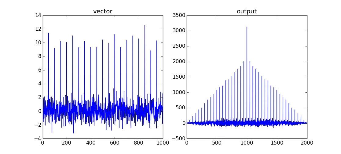
这将返回一个具有最大值的梳形/沙函数，当两个数据集重叠时，它会达到最大值。由于这是一种自相关，因此两个输入信号之间不会有“滞后”。因此，相关的最大值为vector.size-1。

如果您只想获取重叠数据的相关值，则可以使用mode='valid'。

- ebarr

---

这是一个老问题，但因为我有同样的疑问，所以我无法理解我得出了什么结论。我的报告中是否存在自相关性？我该如何翻译输出结果？ - hephestos

Answer 2

目前我只能评论 numpy.correlate。它是一个强大的工具。我使用它有两个目的。第一个是在另一个模式中查找模式：

import numpy as np
import matplotlib.pyplot as plt

some_data = np.random.uniform(0,1,size=100)
subset = some_data[42:50]

mean = np.mean(some_data)
some_data_normalised = some_data - mean
subset_normalised = subset - mean

correlated = np.correlate(some_data_normalised, subset_normalised)
max_index = np.argmax(correlated)  # 42 !

我使用它的第二个用途（以及如何解释结果）是用于频率检测：

hz_a = np.cos(np.linspace(0,np.pi*6,100))
hz_b = np.cos(np.linspace(0,np.pi*4,100))

f, axarr = plt.subplots(2, sharex=True)

axarr[0].plot(hz_a)
axarr[0].plot(hz_b)
axarr[0].grid(True)

hz_a_autocorrelation = np.correlate(hz_a,hz_a,'same')[round(len(hz_a)/2):]
hz_b_autocorrelation = np.correlate(hz_b,hz_b,'same')[round(len(hz_b)/2):]

axarr[1].plot(hz_a_autocorrelation)
axarr[1].plot(hz_b_autocorrelation)
axarr[1].grid(True)

plt.show()

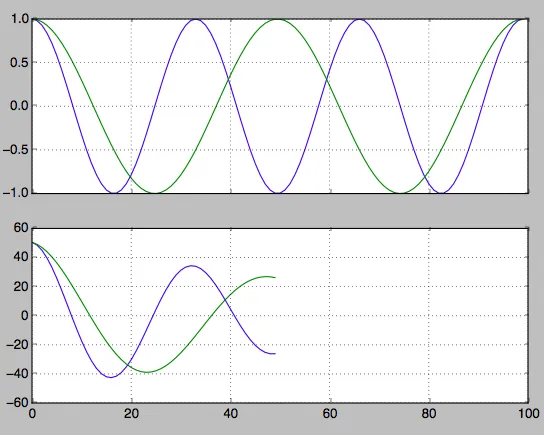
找到第二个峰值的索引。从这里可以倒推出频率。

first_min_index = np.argmin(hz_a_autocorrelation)
second_max_index = np.argmax(hz_a_autocorrelation[first_min_index:])
frequency = 1/second_max_index

- AJP

---

这真的很有帮助。我可以问一下，为什么要取平均值？它看起来像是移动数据，但相关性是曲线而不是值，对吗？ - user-2147482637

@user-2147482637 很好的问题。对此会有一个好答案，除了如果您不减去原始信号的平均值，它就无法工作。 - AJP

@user-2147482637 以下答案解释了为什么要减去平均值，但这个人选择减去均方根(RMS)，在我看来实现了基本相同的结果: https://dev59.com/KKrka4cB1Zd3GeqPeXxs#49742901 - LolPython

Answer 3

在阅读所有教科书的定义和公式后，对于初学者来说，仅仅看到如何从一个中推导出另一个是很有用的。首先，重点关注仅涉及两个向量之间的简单情况。

import numpy as np

arrayA = [ .1, .2, .4 ]
arrayB = [ .3, .1, .3 ]

np.corrcoef( arrayA, arrayB )[0,1] #see Homework bellow why we are using just one cell
>>> 0.18898223650461365

def my_corrcoef( x, y ):    
    mean_x = np.mean( x )
    mean_y = np.mean( y )
    std_x  = np.std ( x )
    std_y  = np.std ( y )
    n      = len    ( x )
    return np.correlate( x - mean_x, y - mean_y, mode = 'valid' )[0] / n / ( std_x * std_y )

my_corrcoef( arrayA, arrayB )
>>> 0.1889822365046136

作业:

• 将示例扩展到两个以上的向量，这就是为什么corrcoef返回矩阵的原因。
• 查看np.correlate在不同于'valid'的模式下做了什么。
• 查看scipy.stats.pearsonr在（arrayA，arrayB）上的操作。

还有一个提示：请注意，在此输入中以“valid”模式使用的np.correlate只是一个点积（与上面的my_corrcoef最后一行进行比较）：

def my_corrcoef1( x, y ):    
    mean_x = np.mean( x )
    mean_y = np.mean( y )
    std_x  = np.std ( x )
    std_y  = np.std ( y )
    n      = len    ( x )
    return (( x - mean_x ) * ( y - mean_y )).sum() / n / ( std_x * std_y )

my_corrcoef1( arrayA, arrayB )
>>> 0.1889822365046136

- ivaylo_iliev

---

正确答案应该是这个，因为它涉及了这两个函数之间的连接。 - David

np.correlate和归一化的讨论缺失了吗？ - user2183336

Answer 4

如果您对 int 向量的结果感到困惑，那可能是由于溢出所致：

>>> a = np.array([4,3,2,0,0,10000,0,0], dtype='int16')
>>> np.correlate(a,a[:3], mode='valid')
array([    29,     18,      8,  20000,  30000, -25536], dtype=int16)

怎么回事？

29 = 4*4 + 3*3 + 2*2
18 = 4*3 + 3*2 + 2*0
 8 = 4*2 + 3*0 + 2*0
...
40000 = 4*10000 + 3*0 + 2*0 shows up as 40000 - 2**16 = -25536

- Rainald62

Answer 5

免责声明：这不会为“如何解释”提供答案，但是介绍了两者之间的区别：

它们之间的区别

Pearson乘积矩相关系数 (np.corrcoef) 是一个 交叉相关 (np.correlate) 的标准化版本， （来源）

因此，np.corrcoef 总是在 -1..+1 的范围内，因此我们可以更好地比较不同的数据。

让我举个例子

import numpy as np
import matplotlib.pyplot as plt

# 1. We make y1 and add noise to it
x = np.arange(0,100)
y1 = np.arange(0,100) + np.random.normal(0, 10.0, 100)

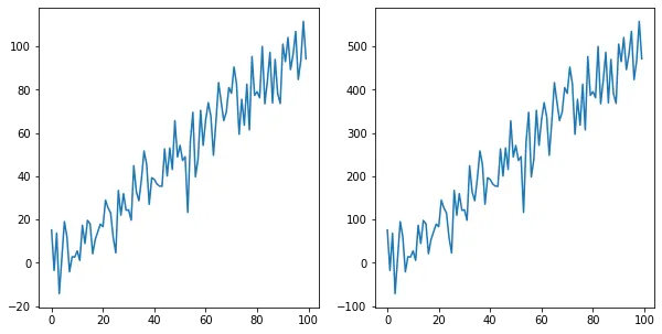
# 2. y2 is exactly y1, but 5 times bigger
y2 = y1 * 5

# 3. By looking at the plot we clearly see that the two lines have the same shape
fig, axs = plt.subplots(1,2, figsize=(10,5))
axs[0].plot(x,y1)
axs[1].plot(x,y2)
fig.show()

# 4. cross-correlation can be misleading, because it is not normalized
print(f"cross-correlation y1: {np.correlate(x, y1)[0]}")
print(f"cross-correlation y2: {np.correlate(x, y2)[0]}")
>>> cross-correlation y1 332291.096
>>> cross-correlation y2 1661455.482

# 5. however, the coefs show that the lines have equal correlations with x
print(f"pearson correlation coef y1: {np.corrcoef(x, y1)[0,1]}")
print(f"pearson correlation coef y2: {np.corrcoef(x, y2)[0,1]}")
>>> pearson correlation coef y1 0.950490
>>> pearson correlation coef y2 0.950490

- tturbo