多组密度图的交集

Question

我正在使用ggplot / easyGgplot2来创建两个组的密度图。我希望有一种度量或指示，可以表现出两个曲线之间的重叠程度。如果能够通过其他解决方案得到各组数据之间更明显的差异度量，也是可以的。

在R中，有没有简便的方法做到这一点呢？例如，使用此示例生成此图：

如何估算两个曲线共同覆盖的区域百分比？

ggplot2.density(data=weight, xName='weight', groupName='sex',
    legendPosition="top",
    alpha=0.5, fillGroupDensity=TRUE )

- Panda

---

如果您对某个度量的群体差异感兴趣（在链接的图像中，它将是“重量”），那么为什么不直接进行t检验呢？ - Chris Watson

根据您的数据需求，您似乎更需要咨询一位统计学家而不是程序员。如果您的问题是关于寻找统计上适当的测试或估计方法，那么您应该在[stats.se]上提问。如果您知道要执行哪个测试，但不知道如何在R中执行它，则应编辑您的问题以使其更清晰明了。 - MrFlick

Answer 1

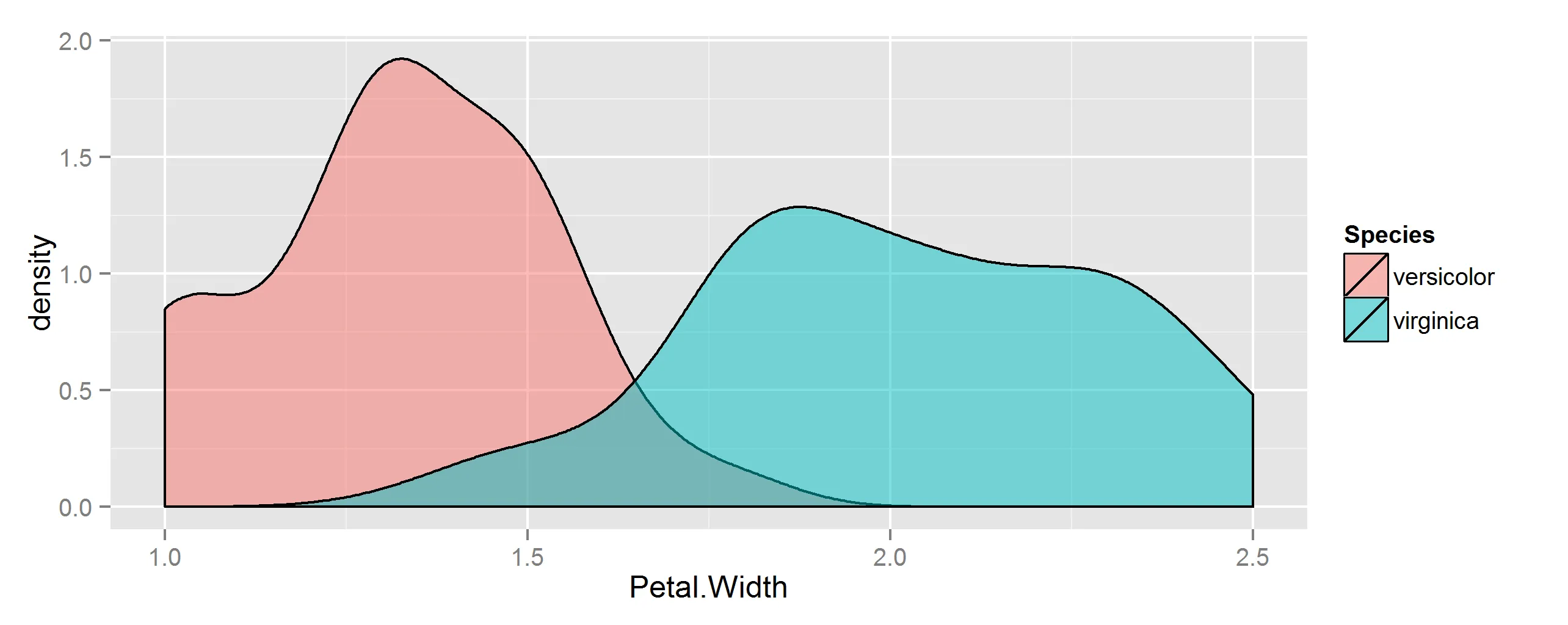
首先，准备一些数据以供使用。这里，我们将查看内置的iris数据集中两个植物物种的花瓣宽度。

## Some sample data from iris
dat <- droplevels(with(iris, iris[Species %in% c("versicolor", "virginica"), ]))

## make a similar graph
library(ggplot2)
ggplot(dat, aes(Petal.Width, fill=Species)) +
  geom_density(alpha=0.5)

要找到交集的区域，您可以使用approxfun逼近描述重叠部分的函数。 然后对其进行积分以得到该区域的面积。 由于它们是密度曲线，因此它们的面积为1（左右），因此积分将是重叠百分比。

## Get density curves for each species
ps <- lapply(split(dat, dat$Species), function(x) {
    dens <- density(x$Petal.Width)
    data.frame(x=dens$x, y=dens$y)
})

## Approximate the functions and find intersection
fs <- sapply(ps, function(x) approxfun(x$x, x$y, yleft=0, yright=0))
f <- function(x) fs[[1]](x) - fs[[2]](x)   # function to minimize (difference b/w curves)
meet <- uniroot(f, interval=c(1, 2))$root  # intersection of the two curves

## Find overlapping x, y values
ps1 <- is.na(cut(ps[[1]]$x, c(-Inf, meet)))
ps2 <- is.na(cut(ps[[2]]$x, c(Inf, meet)))
shared <- rbind(ps[[1]][ps1,], ps[[2]][ps2,])

## Approximate function of intersection
f <- with(shared, approxfun(x, y, yleft=0, yright=0))

## have a look
xs <- seq(0, 3, len=1000)
plot(xs, f(xs), type="l", col="blue", ylim=c(0, 2))

points(ps[[1]], col="red", type="l", lty=2, lwd=2)
points(ps[[2]], col="blue", type="l", lty=2, lwd=2)

polygon(c(xs, rev(xs)), y=c(f(xs), rep(0, length(xs))), col="orange", density=40)

## Integrate it to get the value
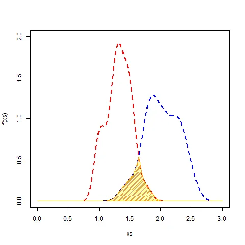
integrate(f, lower=0, upper=3)$value
# [1] 0.1548127

- Rorschach

Answer 2

我喜欢之前的回答，但这个解释可能更易懂，同时我确保使用了一个通用的带宽：

library ( "caTools" )

# Extract common bandwidth
Bw <- ( density ( iris$Petal.Width ))$bw

# Get iris data
Sample <- with ( iris, split ( Petal.Width, Species ))[ 2:3 ]

# Estimate kernel densities using common bandwidth
Densities <- lapply ( Sample, density,
                      bw = bw,
                      n = 512,
                      from = -1,
                      to = 3 )

# Plot
plot( Densities [[ 1 ]], xlim = c ( -1, 3 ),
      col = "steelblue",
      main = "" )
lines ( Densities [[ 2 ]], col = "orange" )

# Overlap
X <- Densities [[ 1 ]]$x
Y1 <- Densities [[ 1 ]]$y
Y2 <- Densities [[ 2 ]]$y

Overlap <- pmin ( Y1, Y2 )
polygon ( c ( X, X [ 1 ]), c ( Overlap, Overlap [ 1 ]),
    lwd = 2, col = "hotpink", border = "n", density = 20) 

# Integrate
Total <- trapz ( X, Y1 ) + trapz ( X, Y2 )
(Surface <- trapz ( X, Overlap ) / Total)
SText <- paste ( sprintf ( "%.3f", 100*Surface ), "%" )
text ( X [ which.max ( Overlap )], 1.2 * max ( Overlap ), SText )

- David.

---

好的答案+1，pmin显然要简单得多！而且trapz是一个很酷的函数。不确定为什么带宽需要相同？ - Rorschach

谢谢！只有一个备注，我不应该将交集面积乘以2才能得到正确的比率吗？ 例如，如果我有两个完全相等的PDF文件，它应该给出100％。但是，将交集区域的面积除以每个PDF区域的总和仅会让我得到50％。我错过了什么吗？ - Panda