MATLAB - 带状区域下 xy 曲线（弯矩分布）

Question

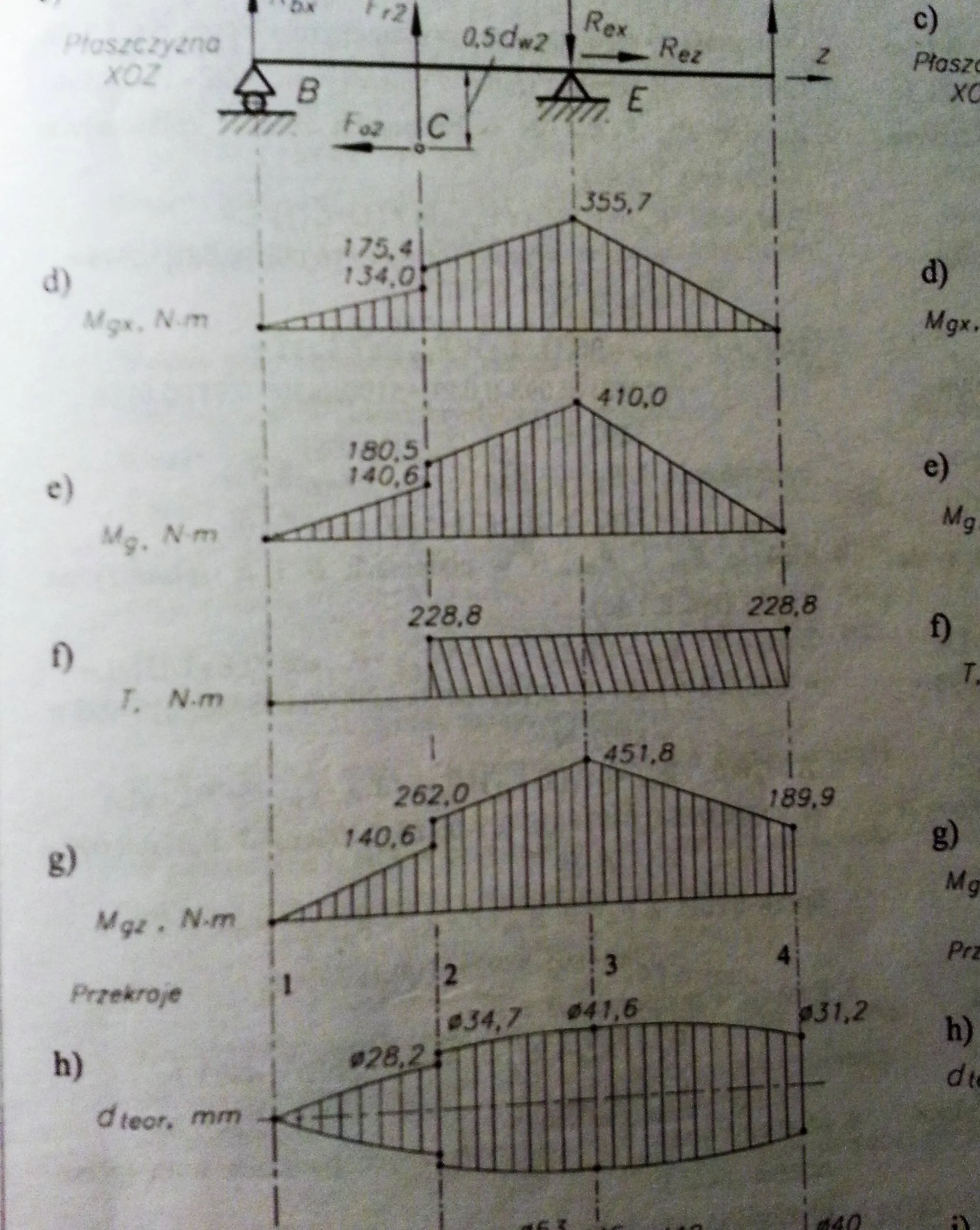
我想要实现的是一个经典的弯矩分布图，可能看起来像这样: 我尝试过使用面积图、xy图和条形图，最后一个接近我所需的——但仍无法满足我的要求。我可以使用任意形式的数据。

- Dominik Roszkowski

---

有许多文件交换条目可以做到这一点。它不是内置功能。这里有一篇很棒的博客文章，重点介绍它们并展示了示例：链接。 - Suever

谢谢，我一定会看看这个方法。 - Dominik Roszkowski

或者，你可以将其分解，先画出轮廓，然后使用stem()而不带标记来绘制线条。一个用于正位，一个用于负位。但前提是你是一种特殊的懒人:D - Andras Deak -- Слава Україні

这似乎很有前途，因为@Suever提出的方法只会产生位图图形。 - Dominik Roszkowski

哦，我还没考虑到那个方面。这样的话，它确实有竞争的机会。 - Andras Deak -- Слава Україні

Answer 1

虽然丹尼尔的回答更加通用，可以用于倾斜的条纹，但这里有一种更简单的解决方案，使用不带标记和基线的stem：

x1 = -3;
x2 = 2;
upfun = @(x) -1/10*(x-x1).*(x-x2);
downfun = @(x) 1/5*(x-x1).*(x-x2);

x_dense = linspace(x1,x2,100);
x_sparse = linspace(x1,x2,20);

%// plot outline
plot(x_dense,upfun(x_dense),'b-',x_dense,downfun(x_dense),'b-');
hold on;
%// plot stripes
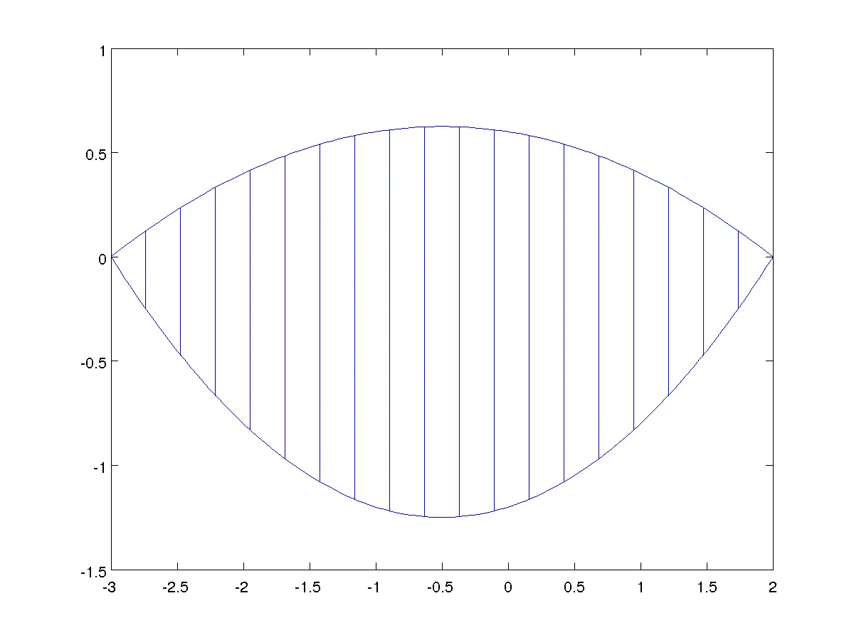
stem(x_sparse,upfun(x_sparse),'b','marker','none','showbaseline','off');
stem(x_sparse,downfun(x_sparse),'b','marker','none','showbaseline','off');

结果：

这是一个显示结果的图片。

- Andras Deak -- Слава Україні

---

谢谢，这个运行得很好。 - Dominik Roszkowski

Answer 2

我会手动生成您想要的行来解决它。

%some example plot
x1 = -3;
x2 = 2;
upfun = @(x) -1/10*(x-x1).*(x-x2);
downfun = @(x) 1/5*(x-x1).*(x-x2);
%set slope you want. Inf for vertical lines
slope=inf;

x_dense = linspace(x1,x2,100);
x_sparse = linspace(x1,x2,20);

%plotting it without the stripes. nan is used not to have unintended lines connecting first and second function
plot([x_dense ,nan,x_dense ],[upfun(x_dense),nan,downfun(x_dense)])

x_stripes=nan(size(x_sparse).*[3,1]);
y_stripes=nan(size(x_sparse).*[3,1]);

if slope==inf
    %vertical lines, no math needed to know the x-value.
    x_stripes(1,:)=x_sparse;
    x_stripes(2,:)=x_sparse;
else
    %intersect both functions with the sloped stripes to know where they
    %end
    for stripe=1:numel(x_sparse)
        x_ax=x_sparse(stripe);
        x_stripes(1,stripe)=fzero(@(x)(upfun(x)-slope*(x-x_ax)),x_ax);
        x_stripes(2,stripe)=fzero(@(x)(downfun(x)-slope*(x-x_ax)),x_ax);
    end
end
y_stripes(1,:)=upfun(x_stripes(1,:));
y_stripes(2,:)=downfun(x_stripes(2,:));
x_stripes=reshape(x_stripes,1,[]);
y_stripes=reshape(y_stripes,1,[]);
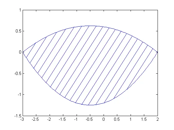
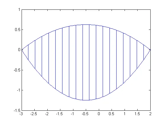
plot([x_dense ,nan,x_dense,nan,x_stripes],[upfun(x_dense),nan,downfun(x_dense),nan,y_stripes])

斜率为1的示例

斜率为无穷大的示例

- Daniel

---

你尝试过画斜条纹吗？你的手动版本可以很容易地实现这一点（不像stem）。 - Andras Deak -- Слава Україні

这可能是可能的，但需要计算线之间的交点。特别是对于像g)这样的情况，斜条纹可能会被切成两半。我不使用stem的主要原因是为了将所有内容保持在一个数据系列中，以便后续步骤（如添加图例）更简单。 - Daniel

你说得对，我没有考虑到像 g) 这样的情况。我们不必担心图例，它们的 行为 可以被禁用。但我知道这只是一个例子 :) 我想这也取决于 OP 需要什么。 - Andras Deak -- Слава Україні

@AndrasDeak：比我最初想象的要简单，至少在忽略g)这样的情况时是这样的。 - Daniel