我有一个矩阵数据,想用热图可视化它。行代表物种,所以我想在行旁边显示系统发生树,并按照树的顺序重新排列热图中的行。我知道R语言中的heatmap函数可以创建层次聚类热图,但如何使用我的系统发生聚类替代绘图中默认创建的距离聚类呢?
如何使用固定的外部分层聚类创建热图
6
- RNA
4
6个回答
13
首先,您需要使用包ape将数据读入为phylo对象。
library(ape)
dat <- read.tree(file="your/newick/file")
#or
dat <- read.tree(text="((A:4.2,B:4.2):3.1,C:7.3);")
以下内容仅适用于超度树。接下来的步骤是将您的系统发育树转换为类
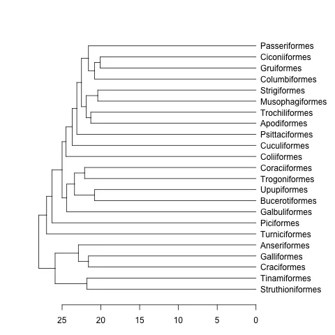
dendrogram。这里提供一个例子:data(bird.orders) #This is already a phylo object
hc <- as.hclust(bird.orders) #Compulsory step as as.dendrogram doesn't have a method for phylo objects.
dend <- as.dendrogram(hc)
plot(dend, horiz=TRUE)
mat <- matrix(rnorm(23*23),nrow=23, dimnames=list(sample(bird.orders$tip, 23), sample(bird.orders$tip, 23))) #Some random data to plot
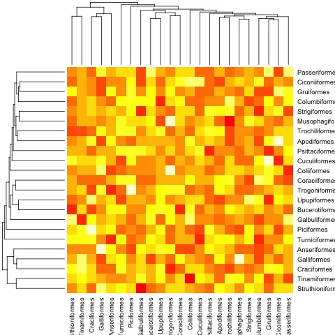
首先,我们需要根据系统发育树的顺序对矩阵进行排序:
ord.mat <- mat[bird.orders$tip,bird.orders$tip]
然后将其输入到
heatmap中:heatmap(ord.mat, Rowv=dend, Colv=dend)
编辑:这里有一个处理超度量树和非超度量树的函数。
heatmap.phylo <- function(x, Rowp, Colp, ...){
    # x numeric matrix
    # Rowp: phylogenetic tree (class phylo) to be used in rows
    # Colp: phylogenetic tree (class phylo) to be used in columns
    # ... additional arguments to be passed to image function
    x <- x[Rowp$tip, Colp$tip]
    xl <- c(0.5, ncol(x)+0.5)
    yl <- c(0.5, nrow(x)+0.5)
    layout(matrix(c(0,1,0,2,3,4,0,5,0),nrow=3, byrow=TRUE),
                  width=c(1,3,1), height=c(1,3,1))
    par(mar=rep(0,4))
    plot(Colp, direction="downwards", show.tip.label=FALSE,
               xlab="",ylab="", xaxs="i", x.lim=xl)
    par(mar=rep(0,4))
    plot(Rowp, direction="rightwards", show.tip.label=FALSE,
               xlab="",ylab="", yaxs="i", y.lim=yl)
    par(mar=rep(0,4), xpd=TRUE)
    image((1:nrow(x))-0.5, (1:ncol(x))-0.5, x,
           xaxs="i", yaxs="i", axes=FALSE, xlab="",ylab="", ...)
    par(mar=rep(0,4))
    plot(NA, axes=FALSE, ylab="", xlab="", yaxs="i", xlim=c(0,2), ylim=yl)
    text(rep(0,nrow(x)),1:nrow(x),Rowp$tip, pos=4)
    par(mar=rep(0,4))
    plot(NA, axes=FALSE, ylab="", xlab="", xaxs="i", ylim=c(0,2), xlim=xl)
    text(1:ncol(x),rep(2,ncol(x)),Colp$tip, srt=90, pos=2)
    }
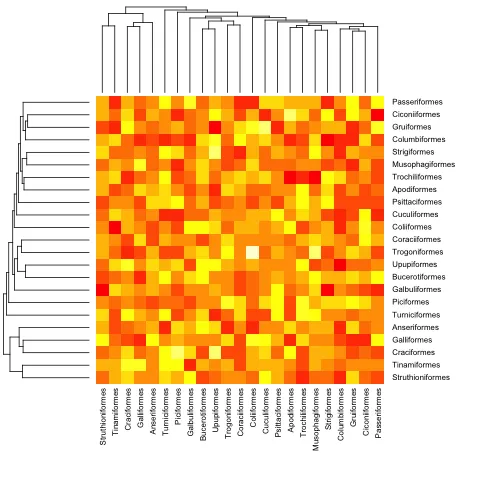
这是与之前(超度量)示例相同的:
heatmap.phylo(mat, bird.orders, bird.orders)
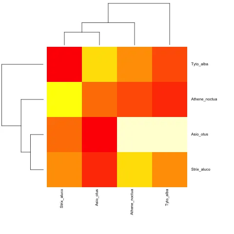
而对于非超度量的情况:
cat("owls(((Strix_aluco:4.2,Asio_otus:4.2):3.1,Athene_noctua:7.3):6.3,Tyto_alba:13.5);",
    file = "ex.tre", sep = "\n")
tree.owls <- read.tree("ex.tre")
mat2 <- matrix(rnorm(4*4),nrow=4,
             dimnames=list(sample(tree.owls$tip,4),sample(tree.owls$tip,4)))
is.ultrametric(tree.owls)
[1] FALSE
heatmap.phylo(mat2,tree.owls,tree.owls)
- plannapus
6
有趣的
heatmap.phylo 函数!这是一种独立于deprogram概念的新方法!我非常确定可以将其转换为网格世界!+10!我相信我可以将其转换为网格包(lattice和grid,不确定是否适用于ggplot2)。 - agstudy没有对超度量树的限制,这非常棒。谢谢你,plannapus! - RNA
我遇到了以下问题:在我的数据上运行
heatmap.phylo(c, d1, d2)时出现错误:Error in image.default((1:ncol(x)) - 0.5, (1:nrow(x)) - 0.5, x, xaxs = "i", : dimensions of z are not length(x)(-1) times length(y)(-1)。我检查了矩阵维度和两棵树的末端长度,它们确实是一致的。你有什么想法可能是问题所在吗?谢谢。 - RNA我已经解决了。在你的
heatmap.phylo() 中,image 函数中的 ncol 和 nrow 被交换了。我已经纠正了它。 - RNA不错的
heatmap.phylo()函数。然而,当我尝试按照您的示例操作时,出现以下错误信息:
Error in plot.default(0, type = "n", xlim = x.lim, ylim = y.lim, xlab = "", : formal argument "xlab" matched by multiple actual arguments。
我不知道错误可能来自哪里,因为我只是将您的示例复制/粘贴到这里,用于非超度量树...有什么想法吗? - Antonio Canepa1@AntonioCanepa 我写了那个函数已经有7年了,我想
ape包自那时起改变了他们的代码来绘制系统发育树。只需在heatmap.phylo代码的第13行和第16行中摆脱xlab=''和ylab=''即可正常工作。 - plannapus3
首先,我会创建一个可重现的示例。如果没有数据,我们就只能猜测您想要什么。因此,请尽量做得更好(特别是您已确认用户)。例如,您可以按以下方式创建newick格式的树:
tree.text='(((XXX:4.2,ZZZ:4.2):3.1,HHH:7.3):6.3,AAA:13.6);'
和@plannpus一样,我正在使用ape将这棵树转换为hclust类。不幸的是,看起来我们只能将超度量树转换为hclust类:从根到每个末端的距离相同。
library(ape)
tree <- read.tree(text='(((XXX:4.2,ZZZ:4.2):3.1,HHH:7.3):6.3,AAA:13.6);')
is.ultrametric(tree)
hc <- as.hclust.phylo(tree)
然后我使用 latticeExtra 的 dendrogramGrob 来绘制我的树形图,使用 lattice 的 levelplot 来绘制热力图。
library(latticeExtra)
dd.col <- as.dendrogram(hc)
col.ord <- order.dendrogram(dd.col)
mat <- matrix(rnorm(4*4),nrow=4)
colnames(mat) <- tree$tip.label
rownames(mat) <- tree$tip.label
levelplot(mat[tree$tip,tree$tip],type=c('g','p'),
          aspect = "fill",
          colorkey = list(space = "left"),
          legend =
            list(right =
                   list(fun = dendrogramGrob,
                        args =
                          list(x = dd.col,
                               side = "right",
                               size = 10))),
          panel=function(...){
            panel.fill('black',alpha=0.2)
            panel.levelplot.points(...,cex=12,pch=23)
          }
)
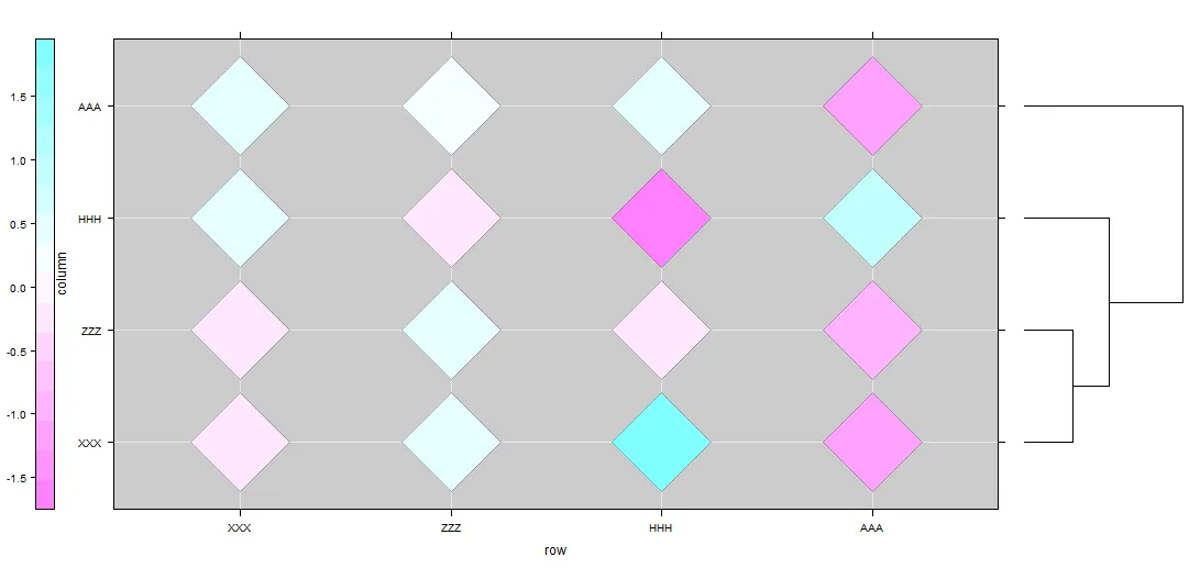
- agstudy
2
+1 像往常一样,非常好。稍后我会尝试看看是否能找到非超度量树的简单解决方法。 - plannapus
你如何调整系统发育图和面板之间的间距? - Daijiang Li
1
我根据plannapus的答案进行了修改,以处理多个树(在此过程中删去了一些我不需要的选项):
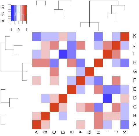
library(ape)

heatmap.phylo <- function(x, Rowp, Colp, breaks, col, denscol="cyan", respect=F, ...){
    # x numeric matrix
    # Rowp: phylogenetic tree (class phylo) to be used in rows
    # Colp: phylogenetic tree (class phylo) to be used in columns
    # ... additional arguments to be passed to image function

    scale01 <- function(x, low = min(x), high = max(x)) {
        x <- (x - low)/(high - low)
        x
    }

    col.tip <- Colp$tip
    n.col <- 1
    if (is.null(col.tip)) {
        n.col <- length(Colp)
        col.tip <- unlist(lapply(Colp, function(t) t$tip))
        col.lengths <- unlist(lapply(Colp, function(t) length(t$tip)))
        col.fraction <- col.lengths / sum(col.lengths)
        col.heights <- unlist(lapply(Colp, function(t) max(node.depth.edgelength(t))))
        col.max_height <- max(col.heights)
    }

    row.tip <- Rowp$tip
    n.row <- 1
    if (is.null(row.tip)) {
        n.row <- length(Rowp)
        row.tip <- unlist(lapply(Rowp, function(t) t$tip))
        row.lengths <- unlist(lapply(Rowp, function(t) length(t$tip)))
        row.fraction <- row.lengths / sum(row.lengths)
        row.heights <- unlist(lapply(Rowp, function(t) max(node.depth.edgelength(t))))
        row.max_height <- max(row.heights)
    }

    cexRow <- min(1, 0.2 + 1/log10(n.row))
    cexCol <- min(1, 0.2 + 1/log10(n.col))

    x <- x[row.tip, col.tip]
    xl <- c(0.5, ncol(x)+0.5)
    yl <- c(0.5, nrow(x)+0.5)

    screen_matrix <- matrix( c(
        0,1,4,5,
        1,4,4,5,
        0,1,1,4,
        1,4,1,4,
        1,4,0,1,
        4,5,1,4
    ) / 5, byrow=T, ncol=4 )

    if (respect) {
        r <- grconvertX(1, from = "inches", to = "ndc") / grconvertY(1, from = "inches", to = "ndc")
        if (r < 1) {
            screen_matrix <- screen_matrix * matrix( c(r,r,1,1), nrow=6, ncol=4, byrow=T)
        } else {
            screen_matrix <- screen_matrix * matrix( c(1,1,1/r,1/r), nrow=6, ncol=4, byrow=T)
        }
    }


    split.screen( screen_matrix )

    screen(2)
    par(mar=rep(0,4))

    if (n.col == 1) {
        plot(Colp, direction="downwards", show.tip.label=FALSE,xaxs="i", x.lim=xl)
    } else {
        screens <- split.screen( as.matrix(data.frame( left=cumsum(col.fraction)-col.fraction, right=cumsum(col.fraction), bottom=0, top=1)))
        for (i in 1:n.col) {
            screen(screens[i])
            plot(Colp[[i]], direction="downwards", show.tip.label=FALSE,xaxs="i", x.lim=c(0.5,0.5+col.lengths[i]), y.lim=-col.max_height+col.heights[i]+c(0,col.max_height))
        }
    }

    screen(3)
    par(mar=rep(0,4))

    if (n.col == 1) {
        plot(Rowp, direction="rightwards", show.tip.label=FALSE,yaxs="i", y.lim=yl)
    } else {
        screens <- split.screen( as.matrix(data.frame( left=0, right=1, bottom=cumsum(row.fraction)-row.fraction, top=cumsum(row.fraction))) )
        for (i in 1:n.col) {
            screen(screens[i])
            plot(Rowp[[i]], direction="rightwards", show.tip.label=FALSE,yaxs="i", x.lim=c(0,row.max_height), y.lim=c(0.5,0.5+row.lengths[i]))
        }
    }


    screen(4)
    par(mar=rep(0,4), xpd=TRUE)
    image((1:nrow(x))-0.5, (1:ncol(x))-0.5, x, xaxs="i", yaxs="i", axes=FALSE, xlab="",ylab="", breaks=breaks, col=col, ...)

    screen(6)
    par(mar=rep(0,4))
    plot(NA, axes=FALSE, ylab="", xlab="", yaxs="i", xlim=c(0,2), ylim=yl)
    text(rep(0,nrow(x)),1:nrow(x),row.tip, pos=4, cex=cexCol)

    screen(5)
    par(mar=rep(0,4))
    plot(NA, axes=FALSE, ylab="", xlab="", xaxs="i", ylim=c(0,2), xlim=xl)
    text(1:ncol(x),rep(2,ncol(x)),col.tip, srt=90, adj=c(1,0.5), cex=cexRow)

    screen(1)
    par(mar = c(2, 2, 1, 1), cex = 0.75)

    symkey <- T
    tmpbreaks <- breaks
    if (symkey) {
        max.raw <- max(abs(c(x, breaks)), na.rm = TRUE)
        min.raw <- -max.raw
        tmpbreaks[1] <- -max(abs(x), na.rm = TRUE)
        tmpbreaks[length(tmpbreaks)] <- max(abs(x), na.rm = TRUE)
    } else {
        min.raw <- min(x, na.rm = TRUE)
        max.raw <- max(x, na.rm = TRUE)
    }
    z <- seq(min.raw, max.raw, length = length(col))

    image(z = matrix(z, ncol = 1), col = col, breaks = tmpbreaks,
          xaxt = "n", yaxt = "n")
    par(usr = c(0, 1, 0, 1))
    lv <- pretty(breaks)
    xv <- scale01(as.numeric(lv), min.raw, max.raw)
    axis(1, at = xv, labels = lv)

    h <- hist(x, plot = FALSE, breaks = breaks)
    hx <- scale01(breaks, min.raw, max.raw)
    hy <- c(h$counts, h$counts[length(h$counts)])
    lines(hx, hy/max(hy) * 0.95, lwd = 1, type = "s",
          col = denscol)
    axis(2, at = pretty(hy)/max(hy) * 0.95, pretty(hy))
    par(cex = 0.5)
    mtext(side = 2, "Count", line = 2)

    close.screen(all.screens = T)

}

tree <- read.tree(text = "(A:1,B:1);((C:1,D:2):2,E:1);((F:1,G:1,H:2):5,((I:1,J:2):2,K:1):1);", comment.char="")
N <- sum(unlist(lapply(tree, function(t) length(t$tip))))

set.seed(42)
m <- cor(matrix(rnorm(N*N), nrow=N))
rownames(m) <- colnames(m) <- LETTERS[1:N]
heatmap.phylo(m, tree, tree, col=bluered(10), breaks=seq(-1,1,length.out=11), respect=T)
- Michael Kuhn
1
嗨@Michael Kuhn。感谢你的代码。然而,当我尝试遵循它,特别是当我尝试通过执行以下操作创建
tree对象时:tree <- read.tree(text = "(A:1,B:1);((C:1,D:2):2,E:1);((F:1,G:1,H:2):5,((I:1,J:2):2,K:1):1);", comment.char=""),我遇到了这个错误消息Error in if (z[i]) { : missing value where TRUE/FALSE needed。有什么想法吗? - Antonio Canepa0
此热力图的具体应用已经在 plot_heatmap 函数(基于 ggplot2)中被实现,该函数位于 phyloseq 包中,且该包是在GitHub 上公开/免费开发的。这里包括了完整代码和结果的示例:
http://joey711.github.io/phyloseq/plot_heatmap-examples
有一个需要注意的地方,虽然不是你明确要求的,但是phyloseq::plot_heatmap不会为任何轴叠加分层树。有一个很好的理由不基于分层聚类来排序轴,这是因为在节点旋转时,长枝末端的索引仍然可以任意相邻。关于这一点,以及基于非度量多维缩放的替代方法在NeatMap软件包文章中有进一步解释,该软件包也是用R编写的,并使用ggplot2。这种降维(排序)方法适用于phyloseq::plot_heatmap中的系统发育丰度数据。
- Paul 'Joey' McMurdie
3
似乎
plot_heatmap 可以制作一个没有层次聚类树的热图,但无法(如 OP 所请求)按系统发生学进行聚类(或在图旁放置系统发生学树以指示系统发生学)。这样说对吗?还是我漏掉了什么? - ohnoplus实际上,自2014年以来,
phyloseq::plot_heatmap可以根据树中的顺序对热图中的分类单元进行排序。这是通过taxa.order命令实现的,该命令可以采用分类阶层来聚类索引,或者采用索引本身的任意顺序。https://www.rdocumentation.org/packages/phyloseq/versions/1.16.2/topics/plot_heatmap https://github.com/joey711/phyloseq/issues/230 - Paul 'Joey' McMurdie其次,我的观点是OP可能过度规定了他们的请求,不理解为什么按热图通过分层或系统发育树排序可能不是他们想要的,因为这明显不是在数据中显示结构模式的更有效的方法。因此,我提到了NeatMap等内容。 - Paul 'Joey' McMurdie
0
虽然我对phlyoseq::plot_heatmap的建议可以让你完成部分工作,但是强大的"ggtree"包可以做更多,如果你真的想要在树上表示数据。
以下是一些示例,显示在下面的ggtree文档页面的顶部:
http://www.bioconductor.org/packages/3.7/bioc/vignettes/ggtree/inst/doc/advanceTreeAnnotation.html
请注意,我与ggtree dev没有任何关联。我只是该项目的粉丝,并且了解其已经能够实现的功能。- Paul 'Joey' McMurdie
0
与@plannapus沟通后,我修改了代码(只是一些)以删除上面代码中的一些额外的xlab = ""信息。
在这里,您将找到代码。您可以看到有注释的行具有额外的代码,现在新行只是擦除它们。
希望这能帮助像我这样的新用户! :)
heatmap.phylo <- function(x, Rowp, Colp, ...){
    # x numeric matrix
    # Rowp: phylogenetic tree (class phylo) to be used in rows
    # Colp: phylogenetic tree (class phylo) to be used in columns
    # ... additional arguments to be passed to image function
    x <- x[Rowp$tip, Colp$tip]
    xl <- c(0.5, ncol(x) + 0.5)
    yl <- c(0.5, nrow(x) + 0.5)
    layout(matrix(c(0,1,0,2,3,4,0,5,0),nrow = 3, byrow = TRUE),
                  width = c(1,3,1), height = c(1,3,1))
    par(mar = rep(0,4))
    # plot(Colp, direction = "downwards", show.tip.label = FALSE,
    #            xlab = "", ylab = "", xaxs = "i", x.lim = xl)
      plot(Colp, direction = "downwards", show.tip.label = FALSE,
               xaxs = "i", x.lim = xl)
    par(mar = rep(0,4))
    # plot(Rowp, direction = "rightwards", show.tip.label = FALSE,
    #            xlab = "", ylab = "", yaxs = "i", y.lim = yl)
    plot(Rowp, direction = "rightwards", show.tip.label = FALSE,
               yaxs = "i", y.lim = yl)
    par(mar = rep(0,4), xpd = TRUE)
    image((1:nrow(x)) - 0.5, (1:ncol(x)) - 0.5, x,
           #xaxs = "i", yaxs = "i", axes = FALSE, xlab = "", ylab = "", ...)
           xaxs = "i", yaxs = "i", axes = FALSE, ...)
    par(mar = rep(0,4))
    plot(NA, axes = FALSE, ylab = "", xlab = "", yaxs = "i", xlim = c(0,2), ylim = yl)
    text(rep(0, nrow(x)), 1:nrow(x), Rowp$tip, pos = 4)
    par(mar = rep(0,4))
    plot(NA, axes = FALSE, ylab = "", xlab = "", xaxs = "i", ylim = c(0,2), xlim = xl)
    text(1:ncol(x), rep(2, ncol(x)), Colp$tip, srt = 90, pos = 2)
}
- Antonio Canepa
网页内容由stack overflow 提供, 点击上面的可以查看英文原文,
原文链接
原文链接
dput(head(mymatrixdata))的输出粘贴到文本中,可以让其他人轻松重建您数据的一部分,并且更容易为您提供帮助。 - Simon O'Hanlon(A:0.1,B:0.2,(C:0.3,D:0.4):0.5);。 - RNA