通过地球上两个已知点的地理距离来确定未知点的位置。

Question

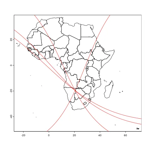
使用我从之前一个问题的接受答案生成的代码https://gis.stackexchange.com/questions/112905/map-location-of-unknown-point-with-distances-to-two-known-points，我不清楚结果是以什么单位产生的？它们似乎不是以经度/纬度的十进制值表示的，而我的输入是。

创建一个小的示例数据框：

group    <- c("A", "B", "C", "D", "E")
distance <- c(709, 2283, 5515, 3035, 4471) ##in km
long     <- c(20.5, 29.4, -14.3, 9.85, -5.5)
lat      <- c(-19.6, 1.6, 10.9, 2.3, 7.5)
df       <- data.frame(group, distance, long, lat)
> df
  group distance  long   lat
1     A      709  20.5 -19.6
2     B     2283  29.4   1.6
3     C     5515 -14.3  10.9
4     D     3035  9.85   2.3
5     E     4471  -5.5   7.5

函数combn创建一个矩阵，其中包含所有成对行比较的索引，并且使用FUN参数，我可以一次使用两个已知点和两个已知距离来确定未知点的位置。

library(geosphere) ##load package for distVincentyEllipsoid function

locations <-  combn(nrow(df), 2, FUN=\(x) {i <- x[1]; j <- x[2];   
  P0 <- df[i, c("long", "lat")]
  x0 <- df[i, "long"]
  y0 <- df[i, "lat"]
  r0 <- df[i, "distance"]
  P1 <- df[j, c("long", "lat")]
  x1 <- df[j, "long"]
  y1 <- df[j, "lat"]
  r1 <- df[j, "distance"]
  d  <- abs(distVincentyEllipsoid(
      P1,
      P0,
      a = 6378137,
      b = 6356752.3142,
      f = 1 / 298.257223563
    ) / 1000)                  ##d in km
  a  <- (r0 ^ 2 - r1 ^ 2 + d ^ 2) / (2 * d)
  h  <- (r0 ^ 2 - a ^ 2) ^ 2
  x2 <- x0 + a * (x1 - x0) / d
  y2 <- y0 + a * (y1 - y0) / d
  x3.1 <- x2 + h * (y1 - y0) / d
  y3.1 <- y2 + h * (x1 - x0) / d
  x3.2 <- x2 - h * (y1 - y0) / d
  y3.2 <- y2 - h * (x1 - x0) / d
  locations <- cbind(x3.1, y3.1, x3.2, y3.2)}  ) ##this creates an array

locations <- matrix(locations, ncol=4, byrow=TRUE) ##change the array into a matrix

这是我希望一对行的输出以矩阵locations的形式呈现的方式：

P0 <- df[df$group == "A", c("long", "lat")] 
x0 <- df[df$group == "A", "long"]
y0 <- df[df$group == "A", "lat"]
r0 <- df[df$group == "A", "distance"] 

P1 <- df[df$group == "B", c("long", "lat")] 
x1 <- df[df$group == "B", "long"]
y1 <- df[df$group == "B", "lat"]
r1 <- df[df$group == "B", "distance"] 

d  <- abs(distVincentyEllipsoid(P1, P0, a = 6378137, b = 6356752.3142, f = 1 / 298.257223563) / 1000)
a  <- (r0 ^ 2 - r1 ^ 2 + d ^ 2) / (2 * d)
h  <- (r0 ^ 2 - a ^ 2) ^ 2
x2 <- x0 + a * (x1 - x0) / d
y2 <- y0 + a * (y1 - y0) / d
x3.1 <- x2 + h * (y1 - y0) / d
y3.1 <- y2 + h * (x1 - x0) / d
x3.2 <- x2 - h * (y1 - y0) / d
y3.2 <- y2 - h * (x1 - x0) / d
locations <- cbind(x3.1, y3.1, x3.2, y3.2)

> locations
           x3.1      y3.1        x3.2       y3.2
[1,] 1243177033 521899766 -1243176990 -521899800

输出每次都是一致的，但我不知道该怎么处理它。我原本期望的是以十进制形式的经度/纬度。

- simpson

---

从文档（distVincentyEllipsoid {geosphere}）中可以得知："距离值与椭球体相同的单位相同（默认为米）"。因此，所有赋给d的值都是以米为单位的。 - undefined

如果轴承是问题，您可以使用maptools::gzAzimuth()。 - undefined

为了快速解决问题，我建议为您感兴趣的区域找到一个等距投影（https://projectionwizard.org/），将您的经纬度转换为平面坐标，使用已知点与未知点之间的距离为两个已知点创建缓冲区，并求得两个圆的交集（请注意，每对点会有两个解）。软件包{sf}提供了`st_points`、`st_transform`、`st_buffer`和`st_intersection`等函数来实现这一过程。另一种方法是使用{geosphere}和`optim`函数来优化（最小化）估计值之间的距离，不过这种方法相对复杂一些。 - undefined

你说得对：投影向导没有提供该区域的投影。你可以谷歌一些其他工具，或者按照这里解释的方法自己选择投影：https://gis.stackexchange.com/questions/364268/choosing-appropriate-projected-coordinate-system-for-africa - undefined

@Chris，我改了标题。希望他能看到并来拯救这一天。 - undefined

Answer 1

宝藏地图的目的是为了模糊，但是通过一组细节，集合成员之间的关系可能会揭示那部分本来更难找到的部分（也许同事会窃取研究想法...）。因此，假设这组细节是有意义的，也许geosphere::greatCircles可以在这里提供帮助。

library(geodata)
library(geosphere)
# using `df` as above
# have a subdirectory in working directory called 'maps`
countries <- world(resolution = 5, path = "maps")
A_mtx = matrix(unlist(df[1, 3:4]), nrow = 1, ncol = 2)
B_mtx = matrix(unlist(df[2, 3:4]), nrow = 1, ncol = 2)
C_mtx = matrix(unlist(df[3, 3:4]), nrow = 1, ncol = 2)
D_mtx = matrix(unlist(df[4, 3:4]), nrow = 1, ncol = 2)
E_mtx = matrix(unlist(df[5, 3:4]), nrow = 1, ncol = 2)
c_codes = country_codes()
# `merge` c_codes with countries
countries = merge(countries, c_codes, by.x = 'GID_0', by.y='ISO3', all.x = TRUE)
png(file = 'greatCircles_to_treasure.png')
plot(countries[which(countries$continent == 'Africa')])
lines(greatCircle(A_mtx, B_mtx, n = 360), col = 'red')
lines(greatCircle(A_mtx, C_mtx, n = 360), col = 'red')
lines(greatCircle(A_mtx, D_mtx, n = 360), col = 'red')
lines(greatCircle(A_mtx, E_mtx, n = 360), col = 'red')
dev.off()

这显示出了希望

但我们可能需要做更多的测试，而测试表明在通过sf之后返回到geosphere函数。 在评论中，建议将缓冲点到距离，这是采取的方法，因为它可以（在某种程度上）回答所有情况== TRUE时。我们还将继续使用修剪为“study_area”的geodata地图。我建议的是，我们正在寻找关于未知起源位置的“大致位置”的共识。关于位置的部分是由使用的标尺和df$distance中的有效数字引入的。

library(sf)
# and library(geodata), and taking the above 'africa' map to study_area
study_area = africa[africa$NAME_0 == 'Angola' | africa$NAME_0 == 'Zambia' | africa$NAME_0 == 'Zimbabwe' | africa$NAME_0 == 'Namibia' | africa$NAME_0 == 'Botswana', ]

# our points
pts_sfc = st_sfc(st_point(A_mtx), st_point(B_mtx), st_point(C_mtx), st_point(D_mtx), st_point(E_mtx))

st_crs(pts_sfc) = 4326
# buffer
A_buffer = st_buffer(pts_sfc[1], dist = df$distance[1] *1000, nQuadSegs = 30)
B_buffer = st_buffer(pts_sfc[2], dist = df$distance[2] *1000, nQuadSegs = 60)
C_buffer = st_buffer(pts_sfc[3], dist = df$distance[3] *1000, nQuadSegs = 180)
D_buffer = st_buffer(pts_sfc[4], dist = df$distance[4] *1000, nQuadSegs = 120)
E_buffer = st_buffer(pts_sfc[5], dist = df$distance[5] *1000, nQuadSegs = 180)
# just pull the boundary using `st_boundry(`
# so, above could be A_boundary = st_boundary(st_buffer(pts_sfc[1]...
A_bound = st_boundary(A_buffer)
B_bound = st_boundary(B_buffer)
C_bound = st_boundary(C_buffer)
D_bound = st_boundary(D_buffer)
E_bound = st_boundary(E_buffer)

# st_intersection
AB_inter = st_intersection(A_bound, B_bound)
AC_inter = st_intersection(A_bound, C_bound)
AD_inter = st_intersection(A_bound, D_bound)
AE_inter = st_intersection(A_bound, E_bound)

检查交叉口输出

AB_inter
Geometry set for 2 features 
Geometry type: GEOMETRY
Dimension:     XY
Bounding box:  xmin: 16.44059 ymin: -18.92567 xmax: 27.26761 ymax: -14.44397
Geodetic CRS:  WGS 84
POINT (27.26761 -18.92567)
LINESTRING (16.44059 -14.44397, 16.44059 -14.53...

# a Point and Linestring

AC_inter
Geometry set for 1 feature 
Geometry type: MULTIPOINT
Dimension:     XY
Bounding box:  xmin: 20.33088 ymin: -26.06643 xmax: 27.17353 ymax: -18.24369
Geodetic CRS:  WGS 84
MULTIPOINT ((27.12648 -18.25086), (27.17353 -18...
# Dang, a Multipoint, how indecisive!
# st_cast this to points
AC_inter_pts = st_cast(st_sfc(AC_inter), 'POINT')
AC_inter_pts
Geometry set for 3 features 
Geometry type: POINT
Dimension:     XY
Bounding box:  xmin: 20.33088 ymin: -26.06643 xmax: 27.17353 ymax: -18.24369
Geodetic CRS:  WGS 84
POINT (27.12648 -18.25086)
POINT (27.17353 -18.24369)
POINT (20.33088 -26.06643)
AD_inter_pts
Geometry set for 2 features 
Geometry type: POINT
Dimension:     XY
Bounding box:  xmin: 15.876 ymin: -24.4339 xmax: 27.26761 ymax: -19.10002
Geodetic CRS:  WGS 84
POINT (27.26761 -19.10002)
POINT (15.876 -24.4339)
> AE_inter_pts
Geometry set for 2 features 
Geometry type: POINT
Dimension:     XY
Bounding box:  xmin: 18.80762 ymin: -25.82576 xmax: 26.89103 ymax: -17.59025
Geodetic CRS:  WGS 84
POINT (26.89103 -17.59025)
POINT (18.80762 -25.82576)

假设在追求共识的过程中，我们有一种直觉，认为起源必须受到限制在某个特定区域内，并且我们想要将我们从上述交集中得到的结果与该区域进行测试。

library(lwgeom)
# hunch is it is somewhere between AD_inter_pts[1] and AE_inter_pts[1]
# create a polygon to intersect
origin_hunch = st_minimum_bounding_circle(st_combine(c(AD_inter_pts[1], AE_inter_pts[1])))
# testing if line string in AB intersects
st_intersects(AB_inter, origin_hunch)
Sparse geometry binary predicate list of length 2, where the predicate
was `intersects'
 1: 1
 2: (empty)
# MULTI-objects will report if one member does, but doesn't say which
st_intersects(AC_inter, origin_hunch)
Sparse geometry binary predicate list of length 1, where the predicate
was `intersects`
 1: 1
#  <- st_cast(st_sfc(some_multi, multi_base_desired(point, line, poly...)
st_intersects(AC_inter_pts, origin_hunch)
Sparse geometry binary predicate list of length 3, where the predicate
was `intersects`
 1: 1
 2: 1
 3: (empty)

有人可能会觉得返回的类型繁多，值得在对象创建过程中退后一步，尝试不同的初始对象来进行交集操作，而不是缓冲边界或凸包。

A_buf_lstring = st_cast(st_convex_hull(A_buffer), 'LINESTRING')
B_buf_lstring = st_cast(st_convex_hull(B_buffer), 'LINESTRING')
st_intersection(A_buf_lstring, B_buf_lstring)
Geometry set for 1 feature 
Geometry type: MULTIPOINT
Dimension:     XY
Bounding box:  xmin: 16.27114 ymin: -19.19564 xmax: 27.32582 ymax: -14.5644
Geodetic CRS:  WGS 84
MULTIPOINT ((27.32582 -19.19564), (16.27114 -14...
st_cast(st_intersection(A_buf_lstring, B_buf_lstring), 'POINT')
Geometry set for 2 features 
Geometry type: POINT
Dimension:     XY
Bounding box:  xmin: 16.27114 ymin: -19.19564 xmax: 27.32582 ymax: -14.5644
Geodetic CRS:  WGS 84
POINT (27.32582 -19.19564)
POINT (16.27114 -14.5644)
# this was our AB_inter previously, now relieved of AB_inter[2]

研究区域的地块

plot(study_area)
plot(A_bound, col = 'red', add = TRUE)
plot(B_bound, col = 'blue', add = TRUE)
plot(C_bound, col = 'green', add = TRUE)
plot(D_bound, col = 'brown', add = TRUE)
plot(E_bound, col = 'red', add = TRUE)
plot(AB_inter_pts[1], col = 'red', pch = 21, cex = 1, bg = 'blue')
plot(AB_inter[1], col = 'red', pch = 21, cex = 1, bg = 'blue')
plot(AC_inter_pts[1], col = 'red', pch = 21, cex = 1, bg = 'green')
plot(AC_inter_pts[2], col = 'red', pch = 21, cex = 1, bg = 'green')
plot(AD_inter_pts[1], col = 'red', pch = 21, cex = 1, bg = 'brown')
plot(AE_inter_pts[1], col = 'red', pch = 21, cex = 1, bg = 'red')

回到共识，未知的起源必须位于A_bound(ary)的东北区块，因为它受到B_bound(ary)的限制。点AB_inter和AD_inter_pts几乎重叠在一起。如果df$distance[3]或[5]有另一个有效数字，即稍微长一点的距离，AC和AE也将几乎重叠在它们上面。

现在我们可以返回到geosphere，检查从交点到大圆起点A:E的距离...

- Chris

---

没有什么会使它们无法发表。目前我不确定为什么距离不同，或者实际上它们是否不同，因为我是从“隆起”的质心进行反测量的，而这本身就是对A:E点（看起来是首都城市）的推测。我也不知道未知是一个点还是一个区域（生态学可能暗示两者都有可能）。如果是在桌子上的地图上用尺量取（未知投影的未知地图），可能会解释这些差异。仅仅令人惊讶的是，第二低距离缓冲区的误差最大。因此，尊重、耐心和谨慎建议进行更多的测试。 - undefined

你提到了我甚至没有考虑到的事情，即从之前的研究者那里得到的距离（公里）可能使用了不同的经纬度十进制人口位置（被描述为大圆距离）。对于我的数据，我确实不得不使用谷歌地球更改人口的经纬度，因为原始的经纬度是从纸质地图上估算出来的，当输入到谷歌地球时实际上可能在海洋中间。你提到的是，我在获取数据时会受到精度的限制，因为我分配了经纬度。那么，这个限制是什么？ - undefined

好的，纸质地图册（我想象着在一张露营桌子旁，手握尺子，喝着金汤力水，时不时被疟疾困扰的情景中，仔细研究着一张地图），但是是哪个纸质地图册，采用了什么投影方式呢？这些测量是你自己进行的还是之前的研究人员进行的？也就是说，这些答案是可以知道的吗（我们只考虑大圆航线和公里数），不同的经纬度可能意味着不同的地图投影（在整个过程中的某个环节）。今天早上我稍微尝试了一下不同的投影方式，但是南非这样的地区，就像罕见疾病一样，是一个被忽视的投影区域。在审稿人提问之前，先把这个问题解决好。 - undefined

之前研究者的数据包括人口和距离（以公里为单位的大圆距离）。我的数据集包括人口和使用谷歌地球选择的经度/纬度十进制数。因此，我无法得知之前研究者使用的纸质地图集和投影方式来定义人口位置，从而计算他的大圆距离。这导致我在估计距离和我所确定的经度/纬度位置之间存在误差，与研究者实际距离不符。在论文中仅仅承认这个限制是否足够？ - undefined

你可以选择等待期刊审阅时提出这个问题（如果他们确实这样做的话，这将取决于所述的方法）。人口似乎固有地是区域性的，即使上面提到的距离有“轻微”差异，假设也很可能成立。AD_inter_pts[1]和AC_inter_pts[2]的st_distance(为95公里（最小外接圆），回到上面的units::drop_units(，df$distance-units::drop_units(，除了df$distance[5]之外，所有距离都在边界圆的范围内（并且可以通过“圆内的位置”来解释）。我只是好奇。你可以写下来。准备好后给我一个作者的预印本链接。 - undefined

Answer 2

这里有一个解决方案，虽然不是最优化的，但是完全可用。

样本数据：

df <- 
data.frame(regionName = c("Anadyr", "Yakutsk", "Magadan"), 
           regionLatitude = c(66.2528, 66.4, 62.9), 
           regionLongitude = c(172.001, 129.167, 153.7),
           dist_from = c(2000000, 3000000, NA) #m
           )

  regionName regionLatitude regionLongitude dist_from
1     Anadyr        66.2528         172.001     2e+06
2    Yakutsk        66.4000         129.167     3e+06
3    Magadan        62.9000         153.700        NA

dist_from - 是一个示例问题 - 距离（以米为单位，从阿纳德尔和雅库茨克）。 我决定选择极地地区，因为你在另一个问题中也问到了安克雷奇和阿纳德尔，并且当绘制区域中心的等距圆时，它们会最容易变形。

首先，我们可以生成由等距点组成的圆：

library(tidyverse)    
steps <- 360 # you can adjust precision and speed of your calculations here
step_angle <- 2 * pi / steps
singularVectors <- 
  tibble(singular_azimuths =
           seq(0, 2 * pi - (step_angle), step_angle)
  ) 


endCoord <- function(lon, lat, bearing, dist, ...){
    bearing <- -1*(bearing / pi * 180 - 90) # conversion of radians to bearing degrees 
    maptools::gcDestination(lon, lat, bearing, dist, ...) %>% 
      c() %>% 
      `names<-`(c("long", "lat"))
}

df_equidistant <- 
crossing(df, singularVectors) %>% 
    data.frame(
    (Vectorize(endCoord, SIMPLIFY = T)(lon = .$regionLongitude, 
                                       lat = .$regionLatitude,
                                       bearing = .$singular_azimuths,
                                       dist = .$dist_from) %>% 
       t 
    )
  )

我们得到了这些等距点的坐标：

head(df_equidistant)
  regionName regionLatitude regionLongitude dist_from singular_azimuths     long      lat
1     Anadyr        66.2528         172.001     2e+06        0.00000000 141.0675 62.84646
2     Anadyr        66.2528         172.001     2e+06        0.01745329 141.3115 62.64018
3     Anadyr        66.2528         172.001     2e+06        0.03490659 141.5596 62.43540
4     Anadyr        66.2528         172.001     2e+06        0.05235988 141.8119 62.23213
5     Anadyr        66.2528         172.001     2e+06        0.06981317 142.0681 62.03041
6     Anadyr        66.2528         172.001     2e+06        0.08726646 142.3281 61.83026

我们可以将它们绘制成圆形：

p <-
ggplot(df_equidistant) +   
geom_point(aes(regionLongitude, regionLatitude, color = regionName), data = df) +   
geom_text(aes(regionLongitude, regionLatitude, label = regionName), data = df, vjust = 1) +   
geom_point(aes(long, lat, color = regionName )) +
scale_color_discrete(name = "Distance from")

我们得到了以下的图表：

这里是一个补充功能（哈弗辛定理），用于计算两个坐标之间的距离：你可以使用这个功能，或者在外部库中找到另一个。

EARTH_RADIUS <- 6378137

mapDistanceHaversine <- function(reg1, reg2) {
  if(any(is.na(c(reg1, reg2)))) return (NA)

  if (all(reg1 == reg2)) return(NA)
    if(reg1[['long']]<0) reg1[['long']] <- reg1[['long']] + 360
    if(reg2[['long']]<0) reg2[['long']] <- reg2[['long']] + 360
    
    reg1 <- reg1 * pi / 180
    reg2 <- reg2 * pi / 180
    
    d <- 2 * asin(sqrt(
      sin((reg2[['lat']] - reg1[['lat']]) / 2)^2 +
        (
          cos(reg1[['lat']]) * 
            cos(reg2[['lat']]) * 
            (sin((reg2[['long']] - reg1[['long']]) / 2)^2)
        )
    ))
    d * EARTH_RADIUS
}

然后我们计算点对之间的距离（这部分以后必须进行优化）：

outerList <- function(a,b, fun) {
  outer(a, b, function(x,y) vapply(seq_along(x), function(i) fun(x[[i]], y[[i]]), numeric(1)))
}

cross_distances <- 
df_equidistant %>% 
  rowwise %>% 
  transmute(eqdc = list(list(long = long, lat = lat) )) %>% 
  pull %>% 
  lapply(unlist) %>% 
  outerList(., ., mapDistanceHaversine) 

我们得到一对点和它们之间的距离：

cross_distances[1:7,1:7]
          [,1]      [,2]      [,3]     [,4]      [,5]      [,6]      [,7]
[1,]        NA  26114.93  52227.98 78337.27 104440.93 130537.07 156623.81
[2,]  26114.93        NA  26114.93 52227.98  78337.27 104440.93 130537.07
[3,]  52227.98  26114.93        NA 26114.93  52227.98  78337.27 104440.93
[4,]  78337.27  52227.98  26114.93       NA  26114.93  52227.98  78337.27
[5,] 104440.93  78337.27  52227.98 26114.93        NA  26114.93  52227.98
[6,] 130537.07 104440.93  78337.27 52227.98  26114.93        NA  26114.93
[7,] 156623.81 130537.07 104440.93 78337.27  52227.98  26114.93        NA

我们找到最小的距离：

point1 <- which(cross_distances == min(cross_distances, na.rm = T), arr.ind = T)

我们有两个点（属于阿纳德尔和雅库茨克圈）：

points
     row col
[1,] 878  64
[2,]  64 878

实际上，这是第一个解决方案（圆A和圆B的交叉点）。

我们需要找到第二个解决方案（选择下一个最小距离之一）：

  point2 <- which(cross_distances == Rfast::nth(cross_distances, 5, na.rm = T), arr.ind = T)

这些解的坐标将是每对点的经度和纬度的平均值：

solutions <-
  rbind(
    df_equidistant[point1[,1],] %>% 
      summarise(long = mean(long),
                lat = mean(lat)),
    df_equidistant[point2[,1],] %>% 
      summarise(long = mean(long),
                lat = mean(lat))
  )

solutions
      long      lat
1 161.7240 53.62795
2 189.2872 78.87114

我们现在可以绘制它们：

p + 
geom_point(aes(x = long, y = lat), solutions, color = "green", size = 3, pch = 17)

附加

优化上述代码的可能方法。

1. 可以将一些小数值分配给steps，然后使用二分搜索singular_azimuths，以在圆点之间获得最小距离。
2. singular_azimuths可以计算到整个圆的一半（方位角-pi/2；方位角+pi/2）。可以使用maptools::gzAzimuth()或类似的函数进行方位角计算。

- asd-tm

---

感谢您逐步解释并沿途解释。从您的代码中：endCoord <- function(lon, lat, bearing, dist, ...){ bearing <- -1*(bearing / pi * 180 - 90) # 将弧度转换为方位角度您从哪里获取到原始的方位信息？我没有这个信息，并且如评论中所讨论的，如果我不知道目的地位置，我不确定如何以无偏的方式生成方位角。 - undefined

@simpson 你好。我生成了从0到2*pi（完整圆）的方位向量。我称它们为“singular_azimuths”。我将生成的方位角转换为方位，因为三角函数中的0表示向右转，角度逆时针增加，我使用弧度来表示它们。方位从北方（顶部）开始，顺时针增加，以度数表示。你可以转换代码并直接生成方位。我使用“singular_azimuts”，因为它们有助于处理欧几里得坐标和方案。 - undefined

你可以尝试使用其他坐标和距离来测试这段代码 - undefined