ggplot2:如何绘制正交回归线?

4

我已经测试了大量参与者在两个不同的视觉感知测试中的表现 - 现在,我想看看两个测试的表现在多大程度上相关。

为了可视化这种相关性,我使用ggplot()在R中绘制散点图,并拟合回归线(使用stat_smooth())。然而,由于我的xy变量都是性能指标,因此在拟合回归线时需要考虑它们两个 - 因此,我不能使用简单的线性回归(使用stat_smooth(method="lm")),而是需要拟合正交回归(或总最小二乘法)。我该如何做到这一点?

我知道我可以在stat_smooth()中指定formula,但我不知道要使用什么公式。从我理解的角度来看,没有一个预设方法(lm,glm,gam,loess,rlm)是适用的。


1
你可以将模型中的slopeintercept传递到geom_abline,或者使用这里展示的方法创建自己的方法。 - user20650
4个回答

8

原来在(x,y)的主成分分析中可以提取斜率和截距,如此处所示。这种方法比较简单,使用基本的R语言即可,并且与使用MethComp中的Deming(...)的结果完全相同。

# same `x and `y` as @user20650's answer
df  <- data.frame(y, x)
pca <- prcomp(~x+y, df)
slp <- with(pca, rotation[2,1] / rotation[1,1])
int <- with(pca, center[2] - slp*center[1])

ggplot(df, aes(x,y)) + 
  geom_point() + 
  stat_smooth(method=lm, color="green", se=FALSE) +
  geom_abline(slope=slp, intercept=int, color="blue")


避免使用额外的包,这是一个很好的方法。还有一个问题,可能更多是关于美学方面的,就是如何限制geom_abline()的长度与数据相同,就像stat_smooth()一样?目前,geom_abline()会延伸到整个图表,而不管数据点是否延伸到整个图表。 - rvrvrv
1
一种方法是使用geom_segment。您知道数据中x范围的最小值和最大值,因此可以使用斜率和截距计算这些限制处的y值,然后使用geom_segment绘制线条。或者,您可以将Deming函数替换为函数f中的不错的prcomp方法。 - user20650

4

注意:我不熟悉这种方法

我认为你只需要将slopeintercept传递给geom_abline,就可以生成拟合线。或者,你可以定义自己的方法传递给stat_smooth(如链接smooth.Pspline wrapper for stat_smooth (in ggplot2)所示)。我使用了MethComp包中建议的链接How to calculate Total least squares in R? (Orthogonal regression)中的Deming函数。

library(MethComp)
library(ggplot2)

# Sample data and model (from ?Deming example) 
set.seed(1)
M <- runif(100,0,5)
# Measurements:
x <-         M + rnorm(100)
y <- 2 + 3 * M + rnorm(100,sd=2)

# Deming regression
mod <- Deming(x,y)

# Define functions to pass to stat_smooth - see mnel's answer at link for details
# Defined the Deming model output as class Deming to define the predict method
# I only used the intercept and slope for predictions - is this correct?
f <- function(formula,data,SDR=2,...){
        M <- model.frame(formula, data)
        d <- Deming(x =M[,2],y =M[,1], sdr=SDR)[1:2]
        class(d) <- "Deming"
        d  
        }

# an s3 method for predictdf (called within stat_smooth)
predictdf.Deming <- function(model, xseq, se, level) {
                         pred <- model %*% t(cbind(1, xseq) )
                         data.frame(x = xseq, y = c(pred))
                         }

ggplot(data.frame(x,y), aes(x, y)) + geom_point() + 
          stat_smooth(method = f, se= FALSE, colour='red', formula=y~x, SDR=1) +  
          geom_abline(intercept=mod[1], slope=mod[2], colour='blue') +
          stat_smooth(method = "lm", se= FALSE, colour='green', formula = y~x)

enter image description here

将拦截和斜率传递给geom_abline,可以产生相同的拟合线(如预期所述)。因此,如果这是正确的方法,则在我看来更容易采用这种方法。

3
“MethComp”包似乎不再维护(已从CRAN中删除)。 Russel88/COEF允许使用method="tls"将正交回归线添加到stat_/geom_summary中。
基于此,以及wikipedia:Deming_regression,我创建了以下函数,允许使用除1之外的噪声比率:

deming.fit <- function(x, y, noise_ratio = sd(y)/sd(x)) {
  if(missing(noise_ratio) || is.null(noise_ratio)) noise_ratio <- eval(formals(sys.function(0))$noise_ratio) # this is just a complicated way to write `sd(y)/sd(x)`
  delta <-  noise_ratio^2
  x_name <- deparse(substitute(x))

  s_yy <- var(y)
  s_xx <- var(x)
  s_xy <- cov(x, y)
  beta1 <- (s_yy - delta*s_xx + sqrt((s_yy - delta*s_xx)^2 + 4*delta*s_xy^2)) / (2*s_xy)
  beta0 <- mean(y) - beta1 * mean(x) 

  res <- c(beta0 = beta0, beta1 = beta1)
  names(res) <- c("(Intercept)", x_name)
  class(res) <- "Deming"
  res
}

deming <- function(formula, data, R = 100, noise_ratio = NULL, ...){
  ret <- boot::boot(
    data = model.frame(formula, data), 
    statistic = function(data, ind) {
      data <- data[ind, ]
      args <- rlang::parse_exprs(colnames(data))
      names(args) <- c("y", "x")
      rlang::eval_tidy(rlang::expr(deming.fit(!!!args, noise_ratio = noise_ratio)), data, env = rlang::current_env())
    },
    R=R
  )
  class(ret) <- c("Deming", class(ret))
  ret  
}

predictdf.Deming <- function(model, xseq, se, level) {
  pred <- as.vector(tcrossprod(model$t0, cbind(1, xseq)))
  if(se) {
    preds <- tcrossprod(model$t, cbind(1, xseq))
    data.frame(
      x = xseq,
      y = pred,
      ymin = apply(preds, 2, function(x) quantile(x, probs = (1-level)/2)),
      ymax = apply(preds, 2, function(x) quantile(x, probs = 1-((1-level)/2)))
    )
  } else {
    return(data.frame(x = xseq, y = pred))
  }
}

# unrelated hlper function to create a nicer plot:
fix_plot_limits <- function(p) p + coord_cartesian(xlim=ggplot_build(p)$layout$panel_params[[1]]$x.range, ylim=ggplot_build(p)$layout$panel_params[[1]]$y.range)
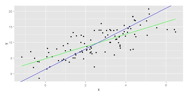
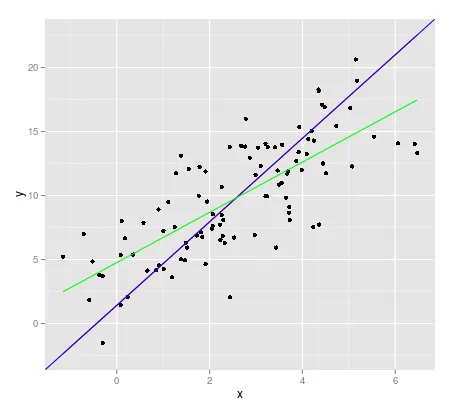
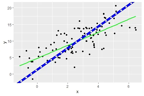
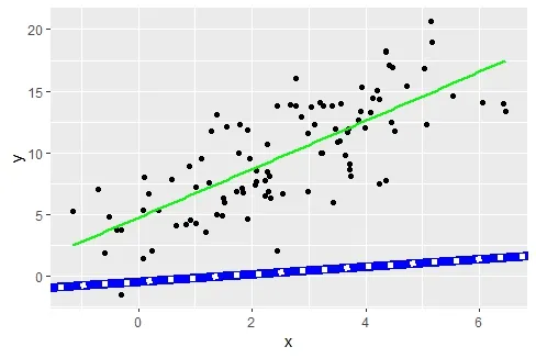

演示:
library(ggplot2)

#devtools::install_github("Russel88/COEF")
library(COEF)

fix_plot_limits(
    ggplot(data.frame(x = (1:5) + rnorm(100), y = (1:5) + rnorm(100)*2), mapping = aes(x=x, y=y)) +
      geom_point()
    ) +
  geom_smooth(method=deming, aes(color="deming"), method.args = list(noise_ratio=2)) +
  geom_smooth(method=lm, aes(color="lm")) +
  geom_smooth(method = COEF::tls, aes(color="tls"))

创建于2019年12月4日,使用reprex package(v0.3.0)。

你知道为什么使用你的函数在 noise_ratio = 1 计算出来的置信区间与 COEF::tls 方法产生的略有不同吗? 附言:非常感谢你的美丽回答,因为它是唯一包括置信区间的回答。 - Cris
1
它们是通过自助法进行估计的,因此是随机的。您可以尝试增加自助样本(R)的数量,并检查是否有助于使它们更相似!如果存在系统性差异,请告诉我! - jan-glx
哦,你说得对!间隔在运行之间略微改变了。谢谢你。 - Cris
1
作者不建议像这样扩展geom_smooth(https://github.com/tidyverse/ggplot2/issues/3132)(但我不确定有什么替代方法)。为了解决ggplot2中predictdf y的非导出问题,可以在yourpackage的.on.load中使用registerS3method("predictdf", "YourClass", yourpackage:::predictdf.YourClass, envir = environment(ggplot2:::predictdf)) - jan-glx
另一个 geom_smooth 技巧。 - jan-glx

1

对于任何感兴趣的人,我已经使用 deming::deming() 函数验证了 jhoward 的解决方案,因为我不熟悉使用 PCA 提取斜率和截距的 jhoward 方法。它们确实产生相同的结果。 Reprex 如下:

# Sample data and model (from ?Deming example) 
set.seed(1)
M <- runif(100,0,5)
# Measurements:
x <-         M + rnorm(100)
y <- 2 + 3 * M + rnorm(100,sd=2)

# Make data.frame()
df <- data.frame(x,y)

# Get intercept and slope using deming::deming()
library(deming)
mod_Dem <- deming::deming(y~x,df)
slp_Dem <- mod_Dem$coefficients[2]
int_Dem <- mod_Dem$coefficients[1]

# Get intercept and slope using jhoward's method
pca <- prcomp(~x+y, df)
slp_jhoward <- with(pca, rotation[2,1] / rotation[1,1])
int_jhoward <- with(pca, center[2] - slp_jhoward*center[1])

# Plot both orthogonal regression lines and simple linear regression line
library(ggplot2)
ggplot(df, aes(x,y)) + 
  geom_point() + 
  stat_smooth(method=lm, color="green", se=FALSE) +
  geom_abline(slope=slp_jhoward, intercept=int_jhoward, color="blue", lwd = 3) +
  geom_abline(slope=slp_Dem, intercept=int_Dem, color = "white", lwd = 2, linetype = 3)

enter image description here

有趣的是,如果在模型中交换x和y的顺序(即mod_Dem <- deming::deming(x~y,df)pca <- prcomp(~y+x, df)),你会得到完全不同的斜率:

enter image description here

我对正交回归的理解非常肤浅,它不把任何一个变量视为自变量或因变量,因此回归线应该不受模型规定方式的影响,例如 y~xx~y。显然我非常错误,我很想听听其他人对我错在哪里的具体原因的看法。


网页内容由stack overflow 提供, 点击上面的
可以查看英文原文,
原文链接