如何在R中制作一个类似Matlab的南瓜图？

Question

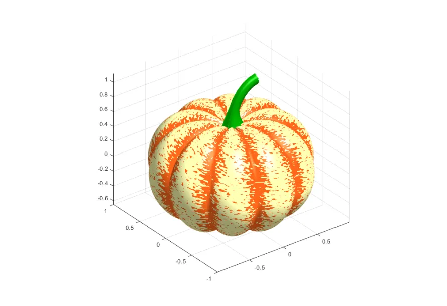
我正在尝试使用以下Matlab代码复制以下可视化效果：

% Pumpkin
[X,Y,Z]=sphere(200);
R=1-(1-mod(0:.1:20,2)).^2/12;
x=R.*X; y=R.*Y; z=Z.*R;
c=hypot(hypot(x,y),z)+randn(201)*.03;
surf(x,y,(.8+(0-(1:-.01:-1)'.^4)*.3).*z,c, 'FaceColor', 'interp', 'EdgeColor', 'none')
% Stem
s = [ 1.5 1 repelem(.7, 6) ] .* [ repmat([.1 .06],1,10) .1 ]';
[t, p] = meshgrid(0:pi/15:pi/2,0:pi/20:pi);
Xs = -(.4-cos(p).*s).*cos(t)+.4;
Zs = (.5-cos(p).*s).*sin(t) + .55;
Ys = -sin(p).*s;
surface(Xs,Ys,Zs,[],'FaceColor', '#008000','EdgeColor','none');
% Style
colormap([1 .4 .1; 1 1 .7])
axis equal
box on
material([.6 1 .3])
lighting g
camlight

我正在研究底部，但进展并不顺利（参见此处）。我目前所拥有的代码如下：

library(pracma)
library(rgl)
sphere <- function(n) {
   dd <- expand.grid(theta = seq(0, 2*pi, length.out = n+1),
                     phi = seq(-pi, pi, length.out = n+1))
   with(dd, 
        list(x = matrix(cos(phi) * cos(theta), n+1),
             y = matrix(cos(phi) * sin(theta), n+1),
             z = matrix(sin(phi), n+1))
        )
}

# Pumpkin
sph<-sphere(200)
X<-sph[[1]]
Y<-sph[[2]]
Z<-sph[[3]]
R<- 1-(1-seq(from=0, to=20,by=0.1))^2/12

x<-R * X
y<-R * Y 
z<-Z * R 

c<-hypot(hypot(x,y),z)+rnorm(201)*0.3
persp3d(x,y,(0.8+(0-seq(from=1, to=-1, by=-0.01)^4)*0.3)*z,col=c)

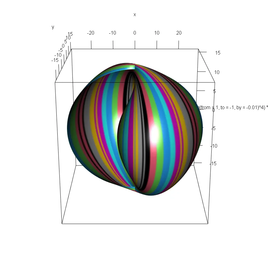
并且它给我以下结果。 我的现有代码出了什么问题？你建议如何修复？

- Bensstats

---

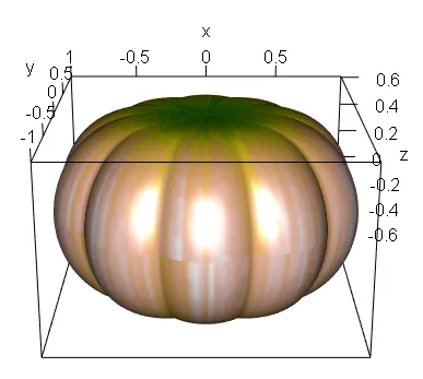
MATLAB代码中似乎有一个mod操作，但在R代码中却没有。@ R<- 1-(1-seq(from=0, to=20,by=0.1))^2/12 - BillBokeey

Answer 1

如@billBokeey所提到的，周期缩放因子缺少mod模运算符函数。

此外，z轴缩放0.8 + (0-seq(from=1, to=-1, by=-0.01)^4) * 0.3与您的sphere函数的输出不匹配。我们可以使用Z[1,]替换seq(from=1, to=-1, by=-0.01)。phi = seq(-pi, pi, length.out = n+1))应该改为seq(-pi/2, pi/2, length.out = n+1))。

最后，颜色c需要转换为RGB代码以用于persp3d。

以下是下面代码的结果。

library(rgl)

sphere <- function(n) {
  dd <- expand.grid(theta = seq(0, 2*pi, length.out = n+1),
                    phi = seq(-pi/2, pi/2, length.out = n+1))
  with(dd, 
       list(x = matrix(cos(phi) * cos(theta), n+1),
            y = matrix(cos(phi) * sin(theta), n+1),
            z = matrix(sin(phi), n+1))
  )
}

# Unit ball
sph <- sphere(200)
X <- sph[[1]]
Y <- sph[[2]]
Z <- sph[[3]]

# scaling
R <- 1 - (1 - seq(from=0, to=20, by=0.1) %% 2) ^ 2 / 12 # Modulo Operator %%
R2 <- 0.8 + (0 - seq(from=1, to=-1, by=-0.01)^4)*0.2 # didn't match with the order of z from sphere function
#R2 <- 0.8 - Z[1,]^4 * 0.2

x <- R * X # scale rows for wavy side
y <- R * Y # scale rows for wavy side
z <- t(R2 * t(Z)) # scale columns by transpose for flat oval shape

# color according to distance to [0,0,0]
hypot_3d <- function(x, y, z) {
  return(sqrt(x^2 + y^2 + z^2))
}
c_ <- hypot_3d(x,y,z) + rnorm(201) * 0.03
color_palette <- terrain.colors(20) # color look-up table
col <- color_palette[ as.numeric(cut(c_, breaks = 20)) ] # assign color to 20 levels of c_

persp3d(x, y, z, color = col, aspect=FALSE)

- Ryan SY Kwan