我有一个 (26424 x 144) 的数组,想使用Python对其执行PCA。然而,网络上没有特定的位置来解释如何完成此任务(有一些网站只是按照自己的方式执行PCA - 没有通用的方法可供查找)。任何能提供任何形式帮助的人都将是伟大的。
11个回答
101
尽管已经有一个答案被接受,但我已发布了我的答案。被接受的答案依赖于一个已弃用函数。此外,这个废弃的函数基于奇异值分解(SVD),虽然完全有效,但与计算主成分分析(PCA)的两种通用技术中更需要的内存和处理器相比,它是更加内存和处理器密集型的。这在这里特别相关,因为原始数据数组的大小很大。使用基于协方差的PCA,计算流程中使用的数组仅为144 x 144而不是26424 x 144(原始数据数组的维度)。
下面是使用SciPy中的linalg模块进行PCA的简单工作实现。因为该实现首先计算协方差矩阵,然后对此数组执行所有后续计算,所以它使用的内存远少于基于SVD的PCA。
(在NumPy中的linalg模块也可以使用以下代码进行,除了导入语句会变成from numpy import linalg as LA之外,代码不需要做任何修改。)
此PCA实现中的两个关键步骤是:
计算协方差矩阵;和
获取该cov矩阵的特征向量和特征值
在下面的函数中,参数dims_rescaled_data指的是重新缩放数据矩阵中所需的维数;此参数默认为只有两个维度,但下面的代码不仅限于两个维度,它可以是任何小于原始数据数组的列数。
def PCA(data, dims_rescaled_data=2):
    """
    returns: data transformed in 2 dims/columns + regenerated original data
    pass in: data as 2D NumPy array
    """
    import numpy as NP
    from scipy import linalg as LA
    m, n = data.shape
    # mean center the data
    data -= data.mean(axis=0)
    # calculate the covariance matrix
    R = NP.cov(data, rowvar=False)
    # calculate eigenvectors & eigenvalues of the covariance matrix
    # use 'eigh' rather than 'eig' since R is symmetric,
    # the performance gain is substantial
    evals, evecs = LA.eigh(R)
    # sort eigenvalue in decreasing order
    idx = NP.argsort(evals)[::-1]
    evecs = evecs[:,idx]
    # sort eigenvectors according to same index
    evals = evals[idx]
    # select the first n eigenvectors (n is desired dimension
    # of rescaled data array, or dims_rescaled_data)
    evecs = evecs[:, :dims_rescaled_data]
    # carry out the transformation on the data using eigenvectors
    # and return the re-scaled data, eigenvalues, and eigenvectors
    return NP.dot(evecs.T, data.T).T, evals, evecs

def test_PCA(data, dims_rescaled_data=2):
    '''
    test by attempting to recover original data array from
    the eigenvectors of its covariance matrix & comparing that
    'recovered' array with the original data
    '''
    _ , _ , eigenvectors = PCA(data, dim_rescaled_data=2)
    data_recovered = NP.dot(eigenvectors, m).T
    data_recovered += data_recovered.mean(axis=0)
    assert NP.allclose(data, data_recovered)


def plot_pca(data):
    from matplotlib import pyplot as MPL
    clr1 =  '#2026B2'
    fig = MPL.figure()
    ax1 = fig.add_subplot(111)
    data_resc, data_orig = PCA(data)
    ax1.plot(data_resc[:, 0], data_resc[:, 1], '.', mfc=clr1, mec=clr1)
    MPL.show()

>>> # iris, probably the most widely used reference data set in ML
>>> df = "~/iris.csv"
>>> data = NP.loadtxt(df, delimiter=',')
>>> # remove class labels
>>> data = data[:,:-1]
>>> plot_pca(data)
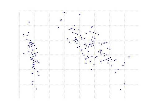
下面的图形是对鸢尾花数据进行PCA函数处理后的可视化结果。可以看到,二维转换清晰地将第一类和第二类、第三类分开(但不能将第二类和第三类分开,这需要另一个维度)。
- doug
16
如何使用此方法检索第一个主成分?谢谢!http://stackoverflow.com/questions/17916837/how-to-get-the-1st-principal-component-by-pca-using-python - Sibbs Gambling
这个有测试过吗?提供的代码无法运行。MPL没有定义,dim1也没有。 - Josh
4@道格,由于你的测试未通过(
m是什么?为什么在返回之前没有定义PCA返回的特征值和特征向量等?等等),因此这样使用起来有点困难... - mmr1@mmr 我已经根据这个答案发布了一个工作示例(在新的答案中)。 - Mark
9为什么不将
NP.dot(evecs.T, data.T).T简化为np.dot(data, evecs)? - Ela782显示剩余11条评论
64
您可以在matplotlib模块中找到一个PCA函数:
import numpy as np
from matplotlib.mlab import PCA

data = np.array(np.random.randint(10,size=(10,3)))
results = PCA(data)
结果将存储PCA的各种参数。这来自于matplotlib的mlab部分,它是与MATLAB语法兼容的兼容层。
编辑: 在博客nextgenetics上我发现了一个精彩的演示,展示了如何使用matplotlib mlab模块执行和显示PCA,请享受并检查该博客!
- EnricoGiampieri
7
Enrico,谢谢。我将用这个3D场景制作3D PCA图。再次感谢。如果出现问题,我会与您联系。 - khan
12@khan,matplot.mlab中的PCA函数已被弃用(http://matplotlib.org/api/mlab_api.html?highlight=mlab#deprecated-functions)。此外,它使用SVD,在OP数据矩阵的大小给定的情况下,这将是一项昂贵的计算。使用协方差矩阵(请参见我下面的答案),您可以通过超过100倍地减少特征向量计算中的矩阵大小。 - doug
1@doug:它并没有被弃用...他们只是删除了文档。我猜测。 - khan
1我很难过,因为这三行代码不起作用! - user2988577
2我认为你想要添加和更改以下命令@user2988577:
import numpy as np 和 data = np.array(np.random.randint(10,size=(10,3)))。然后,我建议你按照这个教程来帮助你学习如何绘图http://blog.nextgenetics.net/?e=42。 - amc显示剩余2条评论
31
使用numpy实现的另一个Python主成分分析。和@doug的思路相同,但那个代码没有运行成功。
from numpy import array, dot, mean, std, empty, argsort
from numpy.linalg import eigh, solve
from numpy.random import randn
from matplotlib.pyplot import subplots, show

def cov(X):
    """
    Covariance matrix
    note: specifically for mean-centered data
    note: numpy's `cov` uses N-1 as normalization
    """
    return dot(X.T, X) / X.shape[0]
    # N = data.shape[1]
    # C = empty((N, N))
    # for j in range(N):
    #   C[j, j] = mean(data[:, j] * data[:, j])
    #   for k in range(j + 1, N):
    #       C[j, k] = C[k, j] = mean(data[:, j] * data[:, k])
    # return C

def pca(data, pc_count = None):
    """
    Principal component analysis using eigenvalues
    note: this mean-centers and auto-scales the data (in-place)
    """
    data -= mean(data, 0)
    data /= std(data, 0)
    C = cov(data)
    E, V = eigh(C)
    key = argsort(E)[::-1][:pc_count]
    E, V = E[key], V[:, key]
    U = dot(data, V)  # used to be dot(V.T, data.T).T
    return U, E, V

""" test data """
data = array([randn(8) for k in range(150)])
data[:50, 2:4] += 5
data[50:, 2:5] += 5

""" visualize """
trans = pca(data, 3)[0]
fig, (ax1, ax2) = subplots(1, 2)
ax1.scatter(data[:50, 0], data[:50, 1], c = 'r')
ax1.scatter(data[50:, 0], data[50:, 1], c = 'b')
ax2.scatter(trans[:50, 0], trans[:50, 1], c = 'r')
ax2.scatter(trans[50:, 0], trans[50:, 1], c = 'b')
show()
这个与更短的输出相同
from sklearn.decomposition import PCA

def pca2(data, pc_count = None):
    return PCA(n_components = 4).fit_transform(data)
据我理解,使用特征值(第一种方法)更适用于高维数据和少样本情况,而使用奇异值分解则更适用于样本数大于维度的情况。
- Mark
8
5使用循环会削弱numpy的优势。通过简单地进行矩阵乘法C = data.dot(data.T),可以更快地计算协方差矩阵。 - Nicholas Mancuso
3嗯,我猜可以使用
numpy.cov。不确定为什么我要包含自己的版本。 - Mark2@Mark
dot(V.T, data.T).T 为什么你这样写,应该等价于 dot(data, V) 吧?_编辑:_啊,我明白了,你可能只是从上面复制过来的。我在dough的回答中添加了一条注释。 - Ela782@Ela782 哦,没错,确实容易多了。 - Mark
1
U = dot(data, V) does not work as data.shape = (150,8) and V.shape = (2,2) with pc_count = 3 - JejeBelfort显示剩余3条评论
15
这是一个需要用到 numpy 的工作。
以下是一篇教程,演示了如何使用 numpy 的内置模块如 mean,cov,double,cumsum,dot,linalg,array,rank 来完成主成分分析。
http://glowingpython.blogspot.sg/2011/07/principal-component-analysis-with-numpy.html
请注意,scipy 在这里也有详细的解释 -
- https://github.com/scikit-learn/scikit-learn/blob/babe4a5d0637ca172d47e1dfdd2f6f3c3ecb28db/scikits/learn/utils/extmath.py#L105
而且 scikit-learn 库还有更多的代码示例 -
https://github.com/scikit-learn/scikit-learn/blob/babe4a5d0637ca172d47e1dfdd2f6f3c3ecb28db/scikits/learn/utils/extmath.py#L105
- Calvin Cheng
3
1我认为链接的glowingpython博客文章中的代码有一些错误,要小心。(请参见博客上的最新评论) - Ela782
@EnricoGiampieri 我同意你的看法 +$\infty$ - Trect
抱歉,我是在讽刺。那个发光的 Python 不起作用。 - Trect
9
这里是scikit-learn选项。使用了StandardScaler这个方法,因为PCA受到比例的影响。
方法1:让scikit-learn选择最少的主成分,以保留至少x%(以下示例中为90%)的方差。
方法二:选择主成分数量(在本例中,选择了2个主成分)。
from sklearn.datasets import load_iris
from sklearn.decomposition import PCA
from sklearn.preprocessing import StandardScaler

iris = load_iris()

# mean-centers and auto-scales the data
standardizedData = StandardScaler().fit_transform(iris.data)

pca = PCA(.90)

principalComponents = pca.fit_transform(X = standardizedData)

# To get how many principal components was chosen
print(pca.n_components_)
方法二:选择主成分数量(在本例中,选择了2个主成分)。
from sklearn.datasets import load_iris
from sklearn.decomposition import PCA
from sklearn.preprocessing import StandardScaler

iris = load_iris()

standardizedData = StandardScaler().fit_transform(iris.data)

pca = PCA(n_components=2)

principalComponents = pca.fit_transform(X = standardizedData)

# to get how much variance was retained
print(pca.explained_variance_ratio_.sum())
来源:https://towardsdatascience.com/pca-using-python-scikit-learn-e653f8989e60
本文介绍如何使用Python中的Scikit-learn库进行主成分分析(PCA)。主成分分析是一种常用于数据降维的技术,它可以减少数据集中的变量数量,同时保留数据集中的重要信息。在本文中,您将学习如何在Python中执行PCA并解释结果。- Michael James Kali Galarnyk
4
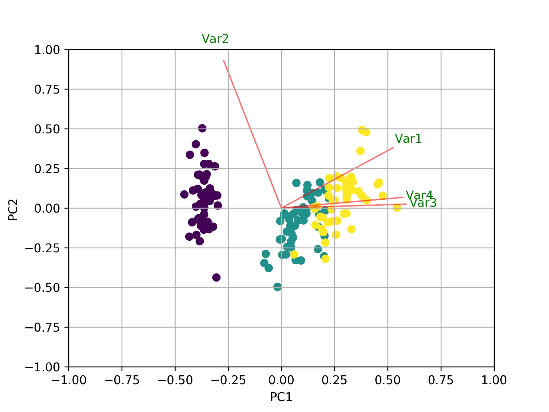
除了其他答案之外,这里有一些使用sklearn和matplotlib绘制biplot的代码。
import numpy as np
import matplotlib.pyplot as plt
from sklearn import datasets
from sklearn.decomposition import PCA
import pandas as pd
from sklearn.preprocessing import StandardScaler

iris = datasets.load_iris()
X = iris.data
y = iris.target
#In general a good idea is to scale the data
scaler = StandardScaler()
scaler.fit(X)
X=scaler.transform(X)

pca = PCA()
x_new = pca.fit_transform(X)

def myplot(score,coeff,labels=None):
    xs = score[:,0]
    ys = score[:,1]
    n = coeff.shape[0]
    scalex = 1.0/(xs.max() - xs.min())
    scaley = 1.0/(ys.max() - ys.min())
    plt.scatter(xs * scalex,ys * scaley, c = y)
    for i in range(n):
        plt.arrow(0, 0, coeff[i,0], coeff[i,1],color = 'r',alpha = 0.5)
        if labels is None:
            plt.text(coeff[i,0]* 1.15, coeff[i,1] * 1.15, "Var"+str(i+1), color = 'g', ha = 'center', va = 'center')
        else:
            plt.text(coeff[i,0]* 1.15, coeff[i,1] * 1.15, labels[i], color = 'g', ha = 'center', va = 'center')
plt.xlim(-1,1)
plt.ylim(-1,1)
plt.xlabel("PC{}".format(1))
plt.ylabel("PC{}".format(2))
plt.grid()

#Call the function. Use only the 2 PCs.
myplot(x_new[:,0:2],np.transpose(pca.components_[0:2, :]))
plt.show()
- seralouk
4
更新: 库
请小心使用以下代码,因为它使用了一个现在已被弃用的库!
现在,在`pca.Y'中,原始数据矩阵是基于主成分基向量的。有关PCA对象的更多详细信息,请查看此处。
你可以使用
matplotlib.mlab.PCA 从2.2版本(2018-03-06)开始已经弃用。
matplotlib.mlab.PCA(在this answer中使用)未被弃用。因此,对于通过Google到达此处的所有人,我将发布一个完整的工作示例,并测试Python 2.7。from matplotlib.mlab import PCA
import numpy
data = numpy.array( [[3,2,5], [-2,1,6], [-1,0,4], [4,3,4], [10,-5,-6]] )
pca = PCA(data)
现在,在`pca.Y'中,原始数据矩阵是基于主成分基向量的。有关PCA对象的更多详细信息,请查看此处。
>>> pca.Y
array([[ 0.67629162, -0.49384752,  0.14489202],
   [ 1.26314784,  0.60164795,  0.02858026],
   [ 0.64937611,  0.69057287, -0.06833576],
   [ 0.60697227, -0.90088738, -0.11194732],
   [-3.19578784,  0.10251408,  0.00681079]])
你可以使用
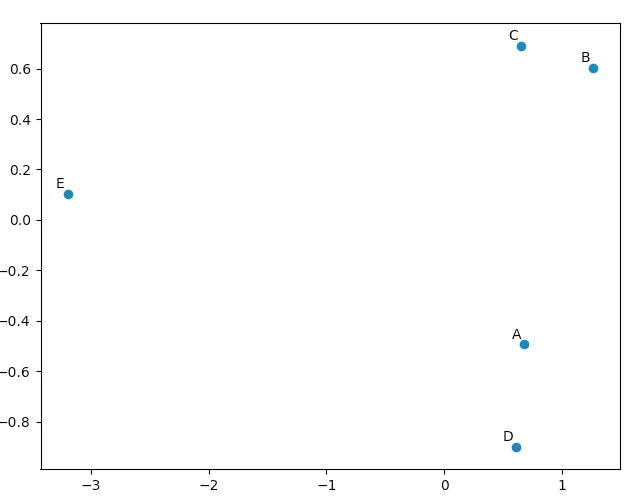
matplotlib.pyplot来绘制这些数据,以便自己确认PCA产生了“好”的结果。 names列表仅用于注释我们的五个向量。import matplotlib.pyplot
names = [ "A", "B", "C", "D", "E" ]
matplotlib.pyplot.scatter(pca.Y[:,0], pca.Y[:,1])
for label, x, y in zip(names, pca.Y[:,0], pca.Y[:,1]):
matplotlib.pyplot.annotate( label, xy=(x, y), xytext=(-2, 2), textcoords='offset points', ha='right', va='bottom' )
matplotlib.pyplot.show()
观察我们的原始向量,我们会发现data[0](“A”)和data[3](“D”)非常相似,data[1](“B”)和data[2](“C”)也是如此。这在我们的PCA转换数据的二维图中得到了体现。
- z80crew
2
我已经编写了一个小脚本用于比较在此处出现的不同主成分分析(PCA)方法:
我已经编写了一个小脚本用于比较在此处出现的不同主成分分析(PCA)方法:
import numpy as np
from scipy.linalg import svd

shape = (26424, 144)
repeat = 20
pca_components = 2

data = np.array(np.random.randint(255, size=shape)).astype('float64')

# data normalization
# data.dot(data.T)
# (U, s, Va) = svd(data, full_matrices=False)
# data = data / s[0]

from fbpca import diffsnorm
from timeit import default_timer as timer

from scipy.linalg import svd
start = timer()
for i in range(repeat):
    (U, s, Va) = svd(data, full_matrices=False)
time = timer() - start
err = diffsnorm(data, U, s, Va)
print('svd time: %.3fms, error: %E' % (time*1000/repeat, err))


from matplotlib.mlab import PCA
start = timer()
_pca = PCA(data)
for i in range(repeat):
    U = _pca.project(data)
time = timer() - start
err = diffsnorm(data, U, _pca.fracs, _pca.Wt)
print('matplotlib PCA time: %.3fms, error: %E' % (time*1000/repeat, err))

from fbpca import pca
start = timer()
for i in range(repeat):
    (U, s, Va) = pca(data, pca_components, True)
time = timer() - start
err = diffsnorm(data, U, s, Va)
print('facebook pca time: %.3fms, error: %E' % (time*1000/repeat, err))


from sklearn.decomposition import PCA
start = timer()
_pca = PCA(n_components = pca_components)
_pca.fit(data)
for i in range(repeat):
    U = _pca.transform(data)
time = timer() - start
err = diffsnorm(data, U, _pca.explained_variance_, _pca.components_)
print('sklearn PCA time: %.3fms, error: %E' % (time*1000/repeat, err))

start = timer()
for i in range(repeat):
    (U, s, Va) = pca_mark(data, pca_components)
time = timer() - start
err = diffsnorm(data, U, s, Va.T)
print('pca by Mark time: %.3fms, error: %E' % (time*1000/repeat, err))

start = timer()
for i in range(repeat):
    (U, s, Va) = pca_doug(data, pca_components)
time = timer() - start
err = diffsnorm(data, U, s[:pca_components], Va.T)
print('pca by doug time: %.3fms, error: %E' % (time*1000/repeat, err))
pca_mark是Mark答案中的pca。
pca_doug是doug答案中的pca。
以下是一个示例输出(但结果非常依赖于数据大小和pca_components,因此建议使用自己的数据运行自己的测试。此外,Facebook的pca针对规范化数据进行了优化,因此在这种情况下它将更快且更准确):
svd time: 3212.228ms, error: 1.907320E-10
matplotlib PCA time: 879.210ms, error: 2.478853E+05
facebook pca time: 485.483ms, error: 1.260335E+04
sklearn PCA time: 169.832ms, error: 7.469847E+07
pca by Mark time: 293.758ms, error: 1.713129E+02
pca by doug time: 300.326ms, error: 1.707492E+02
编辑:
fbpca中的diffsnorm函数计算了一个Schur分解的谱范数误差。
- bendaf
2
准确性与您所称的错误不同。您能否修复此问题并解释一下指标,因为这并不直观,为什么它被认为是可靠的?另外,将Facebook的“随机PCA”与PCA的协方差版本进行比较是不公平的。最后,您是否考虑过某些库标准化输入数据? - ldmtwo
谢谢您的建议,您关于准确性/误差差异的观点是正确的,我已经修改了我的答案。我认为比较随机PCA和基于速度和准确性的PCA是有意义的,因为两者都用于降维。您认为我为什么应该考虑标准化呢? - bendaf
1
这可能是最简单的PCA答案之一,包括易于理解的步骤。假设我们想要保留144个主成分中提供的最大信息,并保留2个主维度。
首先,将您的二维数组转换为数据框:
步骤2:找到原始矩阵X的协方差矩阵S。
步骤四:转化数据。
这个
步骤2:初始化主成分分析(PCA)
步骤三:使用主成分分析(PCA)拟合数据。
这个
首先,将您的二维数组转换为数据框:
import pandas as pd

# Here X is your array of size (26424 x 144)
data = pd.DataFrame(X)
接下来有两种方法可供选择:
方法一:手动计算
步骤1:对X应用列标准化
from sklearn import preprocessing

scalar = preprocessing.StandardScaler()
standardized_data = scalar.fit_transform(data)
步骤2:找到原始矩阵X的协方差矩阵S。
sample_data = standardized_data
covar_matrix = np.cov(sample_data)
第三步:找到S的特征值和特征向量(这里是二维的,因此需要找到2个)
from scipy.linalg import eigh

# eigh() function will provide eigen-values and eigen-vectors for a given matrix.
# eigvals=(low value, high value) takes eigen value numbers in ascending order
values, vectors = eigh(covar_matrix, eigvals=(142,143))

# Converting the eigen vectors into (2,d) shape for easyness of further computations
vectors = vectors.T
步骤四:转化数据。
# Projecting the original data sample on the plane formed by two principal eigen vectors by vector-vector multiplication.

new_coordinates = np.matmul(vectors, sample_data.T)
print(new_coordinates.T)
这个
new_coordinates.T 的大小为 (26424 x 2),含有两个主成分。
方法二:使用Scikit-Learn
步骤1:对X进行列标准化。from sklearn import preprocessing
scalar = preprocessing.StandardScaler()
standardized_data = scalar.fit_transform(data)
步骤2:初始化主成分分析(PCA)
from sklearn import decomposition

# n_components = numbers of dimenstions you want to retain
pca = decomposition.PCA(n_components=2)
步骤三:使用主成分分析(PCA)拟合数据。
# This line takes care of calculating co-variance matrix, eigen values, eigen vectors and multiplying top 2 eigen vectors with data-matrix X.
pca_data = pca.fit_transform(sample_data)
这个
pca_data 的大小将会是 (26424 x 2),其中包含两个主成分。- Dipen Gajjar
1
你好Dipen先生。我正在处理几何问题。我的任务是将几何图形对齐,使得我的主轴与参考轴(x和y)平行或重合。我不知道几何图形旋转的角度。X坐标为:[0.0, 0.87, 1.37, 1.87, 2.73, 3.6, 4.46, 4.96, 5.46, 4.6, 3.73, 2.87, 2.0, 1.5, 1.0, 0.5, 2.37, 3.23, 4.1]。Y坐标为:[0.0, 0.5, -0.37, -1.23, -0.73, -0.23, 0.27, -0.6, -1.46, -1.96, -2.46, -2.96, -3.46, -2.6, -1.73, -0.87, -2.1, -1.6, -1.1]。这些是坐标。请问PCA方法是否有帮助? - Urvesh
0
为了让
def plot_pca(data):正常工作,需要替换这些行。data_resc, data_orig = PCA(data)
ax1.plot(data_resc[:, 0], data_resc[:, 1], '.', mfc=clr1, mec=clr1)
带有行
newData, data_resc, data_orig = PCA(data)
ax1.plot(newData[:, 0], newData[:, 1], '.', mfc=clr1, mec=clr1)
- Edson
网页内容由stack overflow 提供, 点击上面的可以查看英文原文,
原文链接
原文链接
evals--如果您愿意,可以在此处或新问题中发布前几个和总和。并参见维基百科PCA累积能量。 - denisnumpy和/或scipy的基本PCA方法的比较,附有timeit结果。 - djvg