使用GEKKO解决带有约束条件x(0) + x(2) = 0的最优控制问题。

Question

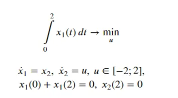
我正在开始学习Gekko并测试最优控制问题。我正在尝试使用Gekko解决以下最优控制问题。

这个问题的解为 (x_1(t) = (t-2)^2 - 2)。如何构建约束条件 x(0) + x(2) = 0？我的代码给出了错误的解决方案。

m = GEKKO(remote=False) # initialize gekko
nt = 101
m.time = np.linspace(0,2,nt) 
#end_loc = nt-1

# Variables
x1 = m.CV(fixed_initial=False)
x2 = m.CV(fixed_initial=False)
x3 = m.Var(value=0)

#u = m.Var(value=0,lb=-2,ub=2)
u = m.MV(fixed_initial=False,lb=-2,ub=2)
u.STATUS = 1


p = np.zeros(nt) # mark final time point
p[-1] = 1.0 
final = m.Param(value=p)

p1 = np.zeros(nt) 
p1[0] = 1.0
p1[-1] = 1.0 
infin = m.Param(value=p1)


# Equations
m.Equation(x1.dt()==x2)
m.Equation(x2.dt()==u)
m.Equation(x3.dt()==x1)

# Constraints 
m.Equation(infin*x1==0)
m.Equation(final*x2==0)

m.Obj(x3*final) # Objective function


#m.fix(x2,pos=end_loc,val=0.0)

m.options.IMODE = 6 # optimal control mode
#m.solve(disp=True) # solve
m.solve(disp=False) # solve


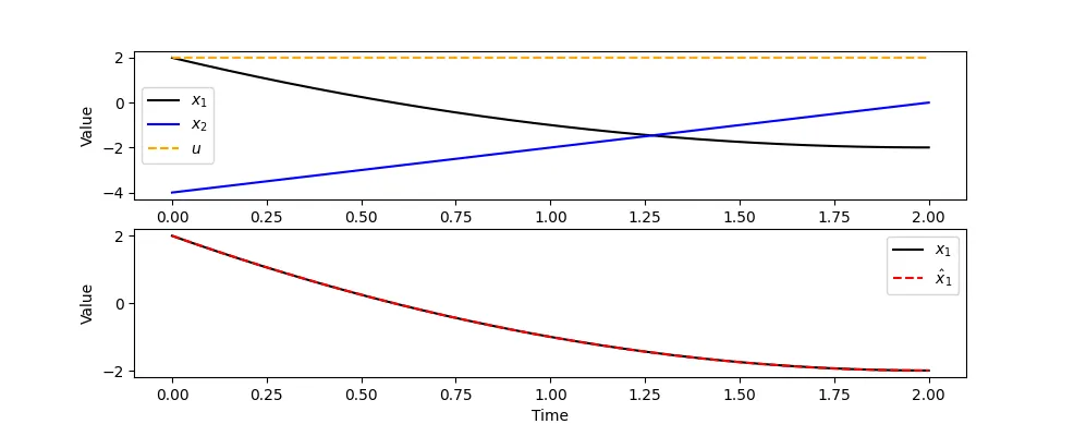
plt.figure(1) # plot results
plt.plot(m.time,x1.value,'k-',label=r'$x_1$')
plt.plot(m.time,x2.value,'b-',label=r'$x_2$')
plt.plot(m.time,x3.value,'g-',label=r'$x_3$')
plt.plot(m.time,u.value,'r--',label=r'$u$')
plt.legend(loc='best')
plt.xlabel('Time')
plt.ylabel('Value')
plt.show()

plt.figure(1) # plot results
plt.plot(m.time,x1.value,'k-',label=r'$x_1$')
plt.plot(m.time,(m.time-2)**2-2,'g--',label=r'$\hat x_1$')
plt.legend(loc='best')
plt.xlabel('Time')
plt.ylabel('Value')
plt.show()

- MRon

---

类似的基准最优控制问题在这里：https://apmonitor.com/do/index.php/Main/DynamicOptimizationBenchmarks。这个问题的独特之处在于 x1(0)+x1(2)=0。 - John Hedengren

Answer 1

使用m.integral或m.vsum()可以创建沿时间方向的时间加权总和或垂直总和。以下是一个复制精确解决方案的示例。

from gekko import GEKKO
import numpy as np
import matplotlib.pyplot as plt

m = GEKKO(remote=True) # initialize gekko
nt = 501
m.time = np.linspace(0,2,nt)

# insert a small time step at the beginning and end
#  for final and initial condition equation x(1e-8)+x(2-1e-8)=0
#  this doesn't change the numerical solution significantly
m.time = np.insert(m.time,1,1e-8)
m.time = np.insert(m.time,len(m.time)-1,2.0-1e-8)
nt += 2

# Variables
x1 = m.Var(fixed_initial=False,lb=-100,ub=100)
x2 = m.Var(fixed_initial=False)

u = m.MV(fixed_initial=False,lb=-2,ub=2)
u.STATUS = 1

p = np.zeros(nt) # mark final time point
p[-2] = 1.0 
final = m.Param(value=p)

q = p.copy()
q[1] = 1.0
final_initial = m.Param(value=q)
xfi = m.Var()
m.Equation(xfi==final_initial*x1)

# Equations
m.Equation(x1.dt()==x2)
m.Equation(x2.dt()==u)
m.Equation(final*m.vsum(xfi)==0)
m.Equation(final*x2==0)

m.Minimize(m.integral(x1)*final) # Objective function

m.options.IMODE = 6 # optimal control mode
m.options.NODES = 2
m.solve(disp=True) # solve

plt.figure(1) # plot results
plt.subplot(2,1,1)
plt.plot(m.time,x1.value,'k-',label=r'$x_1$')
plt.plot(m.time,x2.value,'b-',label=r'$x_2$')
plt.plot(m.time,u.value,'--',color='orange',label=r'$u$')
plt.legend(loc='best')
plt.ylabel('Value')

plt.subplot(2,1,2)
plt.plot(m.time,x1.value,'k-',label=r'$x_1$')
plt.plot(m.time,(m.time-2)**2-2,'r--',label=r'$\hat x_1$')
plt.legend(loc='best')
plt.xlabel('Time')
plt.ylabel('Value')
plt.show()

一个问题是使用x1（1-e8）+x1（2-1e-8）= 0作为约束条件，而不是x1（0）+ x1（2）= 0 。 数值解应该几乎等效，并且1e-8可以进一步减小。

- John Hedengren