我正在使用Matplotlib的自定义投影,但不知道如何在该投影中进行矢量转换(注意:定制投影是兰伯特等面积方位投影,具有赤道方位)。
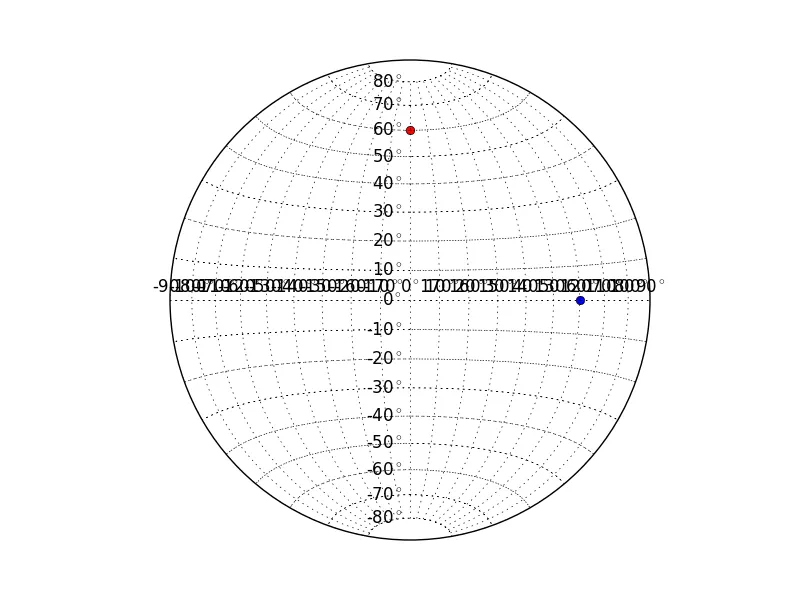
在我的示例中,我想将一点从向北倾斜30度(意味着该点位于赤道60°N)转换为向东倾斜30度的点(意味着它位于本初子午线东60°处)。我希望在矢量转换矩阵的帮助下进行此操作,以便在将来的程序复杂计算中使用。但我真的不明白如何正确获取转换后矢量的长度(或获取该点的正确经纬度)。
我还在学习这个例子,但它使用了略微不同的转换方法: https://github.com/joferkington/mplstereonet/blob/master/mplstereonet/stereonet_math.py 测试文件:
在我的示例中,我想将一点从向北倾斜30度(意味着该点位于赤道60°N)转换为向东倾斜30度的点(意味着它位于本初子午线东60°处)。我希望在矢量转换矩阵的帮助下进行此操作,以便在将来的程序复杂计算中使用。但我真的不明白如何正确获取转换后矢量的长度(或获取该点的正确经纬度)。
我还在学习这个例子,但它使用了略微不同的转换方法: https://github.com/joferkington/mplstereonet/blob/master/mplstereonet/stereonet_math.py 测试文件:
import matplotlib
import matplotlib.pyplot as plt
import numpy as np
from numpy import pi, sin, cos, sqrt, tan, arctan2, arccos

#Internal imports
import projection

def transformVector(geom, raxis, rot):
    """
    Input:
    geom: single point geometry (vector)
    raxis: rotation axis as a vector (vector)
    ([0][1][2]) = (x,y,z) = (Longitude, Latitude, Down)
    rot: rotation in radian

    Returns:
    Array: a vector that has been transformed
    """
    sr = sin(rot)
    cr = cos(rot)
    omcr = 1.0 - cr
    tf = np.array([
        [cr + raxis[0]**2 * omcr,
        -raxis[2] * sr + raxis[0] * raxis[1] * omcr,
        raxis[1] * sr + raxis[0] * raxis[2] * omcr],
        [raxis[2] * sr + raxis[1] * raxis[0] * omcr,
        cr + raxis[1]**2 * omcr,
        -raxis[0] * sr + raxis[1] * raxis[2] * omcr],
        [-raxis[1] * sr + raxis[2] * raxis[0] * omcr,
        raxis[0] * sr + raxis[2] * raxis[1] * omcr,
        cr + raxis[2]**2 * omcr]])

    ar = np.dot(geom, tf)
    return ar

def sphericalToVector(inp_ar):
    """
    Convert a spherical measurement into a vector in cartesian space
    [0] = x (+) east (-) west
    [1] = y (+) north (-) south
    [2] = z (+) down
    """
    ar = np.array([0.0, 0.0, 0.0])
    ar[0] = sin(inp_ar[0]) * cos(inp_ar[1])
    ar[1] = cos(inp_ar[0]) * cos(inp_ar[1])
    ar[2] = sin(inp_ar[1])
    return ar

def vectorToGeogr(vect):
    """
    Returns:
    Array with the components [0] longitude, [1] latitude
    """
    ar = np.array([0.0, 0.0])
    ar[0] = np.arctan2(vect[0], vect[2])
    ar[1] = np.arctan2(vect[1], vect[2])
    ar = ar * pi/2
    return ar

def plotPoint(dip):
    """
    Testfunction for converting, transforming and plotting a point
    """
    plt.subplot(111, projection="lmbrt_equ_area_equ_aspect")

    #Convert to radians
    dip_rad = np.radians(dip)

    #Set rotation to azimuth and convert dip to latitude on north-south axis
    rot = dip_rad[0]
    dip_lat = pi/2 - dip_rad[1]
    plt.plot(0, dip_lat, "ro")
    print(dip_lat, rot)

    #Convert the dip into a vector along the north-south axis
    #x = 0, y = dip
    vect = sphericalToVector([0, dip_lat])
    print(vect, np.linalg.norm(vect))

    #Transfrom the dip to its proper azimuth
    tvect = transformVector(vect, [0,0,1], rot)
    print(tvect, np.linalg.norm(tvect))

    #Transform the vector back to geographic coordinates
    geo = vectorToGeogr(tvect)
    print(geo)
    plt.plot(geo[0], geo[1], "bo")

    plt.grid(True)
    plt.show()

datapoint = np.array([090.0,30])
plotPoint(datapoint)
自定义投影:
import matplotlib
from matplotlib.axes import Axes
from matplotlib.patches import Circle
from matplotlib.path import Path
from matplotlib.ticker import NullLocator, Formatter, FixedLocator
from matplotlib.transforms import Affine2D, BboxTransformTo, Transform
from matplotlib.projections import register_projection
import matplotlib.spines as mspines
import matplotlib.axis as maxis
import matplotlib.pyplot as plt
import numpy as np
from numpy import pi, sin, cos, sqrt, arctan2
# This example projection class is rather long, but it is designed to
# illustrate many features, not all of which will be used every time.
# It is also common to factor out a lot of these methods into common
# code used by a number of projections with similar characteristics
# (see geo.py).

class LambertAxes(Axes):
    """
    A custom class for the Lambert azimuthal equal-area projection
    with equatorial aspect. In geosciences this is also referre to
    as a "Schmidt plot". For more information see:
    http://pubs.er.usgs.gov/publication/pp1395
    """
    # The projection must specify a name.  This will be used be the
    # user to select the projection, i.e. ``subplot(111,
    # projection='lmbrt_equ_area_equ_aspect')``.
    name = 'lmbrt_equ_area_equ_aspect'

    def __init__(self, *args, **kwargs):
        Axes.__init__(self, *args, **kwargs)
        self.set_aspect(1, adjustable='box', anchor='C')
        self.cla()

    def _init_axis(self):
        self.xaxis = maxis.XAxis(self)
        self.yaxis = maxis.YAxis(self)
        # Do not register xaxis or yaxis with spines -- as done in
        # Axes._init_axis() -- until LambertAxes.xaxis.cla() works.
        # self.spines['hammer'].register_axis(self.yaxis)
        self._update_transScale()

    def cla(self):
        """
        Override to set up some reasonable defaults.
        """
        # Don't forget to call the base class
        Axes.cla(self)

        # Set up a default grid spacing
        self.set_longitude_grid(10)
        self.set_latitude_grid(10)
        self.set_longitude_grid_ends(80)

        # Turn off minor ticking altogether
        self.xaxis.set_minor_locator(NullLocator())
        self.yaxis.set_minor_locator(NullLocator())

        # Do not display ticks -- we only want gridlines and text
        self.xaxis.set_ticks_position('none')
        self.yaxis.set_ticks_position('none')

        # The limits on this projection are fixed -- they are not to
        # be changed by the user.  This makes the math in the
        # transformation itself easier, and since this is a toy
        # example, the easier, the better.
        Axes.set_xlim(self, -pi/2, pi/2)
        Axes.set_ylim(self, -pi, pi)

    def _set_lim_and_transforms(self):
        """
        This is called once when the plot is created to set up all the
        transforms for the data, text and grids.
        """
        # There are three important coordinate spaces going on here:
        #
        #    1. Data space: The space of the data itself
        #
        #    2. Axes space: The unit rectangle (0, 0) to (1, 1)
        #       covering the entire plot area.
        #
        #    3. Display space: The coordinates of the resulting image,
        #       often in pixels or dpi/inch.

        # This function makes heavy use of the Transform classes in
        # ``lib/matplotlib/transforms.py.`` For more information, see
        # the inline documentation there.

        # The goal of the first two transformations is to get from the
        # data space (in this case longitude and latitude) to axes
        # space.  It is separated into a non-affine and affine part so
        # that the non-affine part does not have to be recomputed when
        # a simple affine change to the figure has been made (such as
        # resizing the window or changing the dpi).

        # 1) The core transformation from data space into
        # rectilinear space defined in the LambertEqualAreaTransform class.
        self.transProjection = self.LambertEqualAreaTransform()

        # 2) The above has an output range that is not in the unit
        # rectangle, so scale and translate it so it fits correctly
        # within the axes.  The peculiar calculations of xscale and
        # yscale are specific to a Aitoff-Hammer projection, so don't
        # worry about them too much.
        xscale = sqrt(2.0) * sin(0.5 * pi)
        yscale = sqrt(2.0) * sin(0.5 * pi)
        self.transAffine = Affine2D() \
            .scale(0.5 / xscale, 0.5 / yscale) \
            .translate(0.5, 0.5)

        # 3) This is the transformation from axes space to display
        # space.
        self.transAxes = BboxTransformTo(self.bbox)

        # Now put these 3 transforms together -- from data all the way
        # to display coordinates.  Using the '+' operator, these
        # transforms will be applied "in order".  The transforms are
        # automatically simplified, if possible, by the underlying
        # transformation framework.
        self.transData = \
            self.transProjection + \
            self.transAffine + \
            self.transAxes

        # The main data transformation is set up.  Now deal with
        # gridlines and tick labels.

        # Longitude gridlines and ticklabels.  The input to these
        # transforms are in display space in x and axes space in y.
        # Therefore, the input values will be in range (-xmin, 0),
        # (xmax, 1).  The goal of these transforms is to go from that
        # space to display space.  The tick labels will be offset 4
        # pixels from the equator.
        self._xaxis_pretransform = \
            Affine2D() \
            .scale(1.0, pi) \
            .translate(0.0, -pi)
        self._xaxis_transform = \
            self._xaxis_pretransform + \
            self.transData
        self._xaxis_text1_transform = \
            Affine2D().scale(1.0, 0.0) + \
            self.transData + \
            Affine2D().translate(0.0, 4.0)
        self._xaxis_text2_transform = \
            Affine2D().scale(1.0, 0.0) + \
            self.transData + \
            Affine2D().translate(0.0, -4.0)

        # Now set up the transforms for the latitude ticks.  The input to
        # these transforms are in axes space in x and display space in
        # y.  Therefore, the input values will be in range (0, -ymin),
        # (1, ymax).  The goal of these transforms is to go from that
        # space to display space.  The tick labels will be offset 4
        # pixels from the edge of the axes ellipse.
        yaxis_stretch = Affine2D().scale(pi * 2.0, 1.0).translate(-pi, 0.0)
        yaxis_space = Affine2D().scale(1.0, 1.0)
        self._yaxis_transform = \
            yaxis_stretch + \
            self.transData
        yaxis_text_base = \
            yaxis_stretch + \
            self.transProjection + \
            (yaxis_space + \
             self.transAffine + \
             self.transAxes)
        self._yaxis_text1_transform = \
            yaxis_text_base + \
            Affine2D().translate(-8.0, 0.0)
        self._yaxis_text2_transform = \
            yaxis_text_base + \
            Affine2D().translate(8.0, 0.0)

    def get_xaxis_transform(self,which='grid'):
        """
        Override this method to provide a transformation for the
        x-axis grid and ticks.
        """
        assert which in ['tick1','tick2','grid']
        return self._xaxis_transform

    def get_xaxis_text1_transform(self, pixelPad):
        """
        Override this method to provide a transformation for the
        x-axis tick labels.

        Returns a tuple of the form (transform, valign, halign)
        """
        return self._xaxis_text1_transform, 'bottom', 'center'

    def get_xaxis_text2_transform(self, pixelPad):
        """
        Override this method to provide a transformation for the
        secondary x-axis tick labels.

        Returns a tuple of the form (transform, valign, halign)
        """
        return self._xaxis_text2_transform, 'top', 'center'

    def get_yaxis_transform(self,which='grid'):
        """
        Override this method to provide a transformation for the
        y-axis grid and ticks.
        """
        assert which in ['tick1','tick2','grid']
        return self._yaxis_transform

    def get_yaxis_text1_transform(self, pixelPad):
        """
        Override this method to provide a transformation for the
        y-axis tick labels.

        Returns a tuple of the form (transform, valign, halign)
        """
        return self._yaxis_text1_transform, 'center', 'right'

    def get_yaxis_text2_transform(self, pixelPad):
        """
        Override this method to provide a transformation for the
        secondary y-axis tick labels.

        Returns a tuple of the form (transform, valign, halign)
        """
        return self._yaxis_text2_transform, 'center', 'left'

    def _gen_axes_patch(self):
        """
        Override this method to define the shape that is used for the
        background of the plot.  It should be a subclass of Patch.

        In this case, it is a Circle (that may be warped by the axes
        transform into an ellipse).  Any data and gridlines will be
        clipped to this shape.
        """
        return Circle((0.5, 0.5), 0.5)

    def _gen_axes_spines(self):
        return {'lmbrt_equ_area_equ_aspect':mspines.Spine.circular_spine(self,
                                                      (0.5, 0.5), 0.5)}

    # Prevent the user from applying scales to one or both of the
    # axes.  In this particular case, scaling the axes wouldn't make
    # sense, so we don't allow it.
    def set_xscale(self, *args, **kwargs):
        if args[0] != 'linear':
            raise NotImplementedError
        Axes.set_xscale(self, *args, **kwargs)

    def set_yscale(self, *args, **kwargs):
        if args[0] != 'linear':
            raise NotImplementedError
        Axes.set_yscale(self, *args, **kwargs)

    # Prevent the user from changing the axes limits.  In our case, we
    # want to display the whole sphere all the time, so we override
    # set_xlim and set_ylim to ignore any input.  This also applies to
    # interactive panning and zooming in the GUI interfaces.
    def set_xlim(self, *args, **kwargs):
        Axes.set_xlim(self, -pi, pi)
        Axes.set_ylim(self, -pi, pi)
    set_ylim = set_xlim

    def format_coord(self, lon, lat):
        """
        Override this method to change how the values are displayed in
        the status bar.

        In this case, we want them to be displayed in degrees N/S/E/W.
        """
        lon = np.degrees(lon)
        lat = np.degrees(lat)

        #if lat >= 0.0:
        #    ns = 'N'
        #else:
        #    ns = 'S'
        #if lon >= 0.0:
        #    ew = 'E'
        #else:
        #    ew = 'W'
        return "{0} / {1}".format(round(lon,1), round(lat,1))

    class DegreeFormatter(Formatter):
        """
        This is a custom formatter that converts the native unit of
        radians into (truncated) degrees and adds a degree symbol.
        """
        def __init__(self, round_to=1.0):
            self._round_to = round_to

        def __call__(self, x, pos=None):
            degrees = (x / pi) * 180.0
            degrees = round(degrees / self._round_to) * self._round_to
            return "%d\u00b0" % degrees

    def set_longitude_grid(self, degrees):
        """
        Set the number of degrees between each longitude grid.

        This is an example method that is specific to this projection
        class -- it provides a more convenient interface to set the
        ticking than set_xticks would.
        """
        # Set up a FixedLocator at each of the points, evenly spaced
        # by degrees.
        number = (360.0 / degrees) + 1
        self.xaxis.set_major_locator(
            plt.FixedLocator(
                np.linspace(-pi, pi, number, True)[1:-1]))
        # Set the formatter to display the tick labels in degrees,
        # rather than radians.
        self.xaxis.set_major_formatter(self.DegreeFormatter(degrees))

    def set_latitude_grid(self, degrees):
        """
        Set the number of degrees between each longitude grid.

        This is an example method that is specific to this projection
        class -- it provides a more convenient interface than
        set_yticks would.
        """
        # Set up a FixedLocator at each of the points, evenly spaced
        # by degrees.
        number = (180.0 / degrees) + 1
        self.yaxis.set_major_locator(
            FixedLocator(
                np.linspace(-pi / 2.0, pi / 2.0, number, True)[1:-1]))
        # Set the formatter to display the tick labels in degrees,
        # rather than radians.
        self.yaxis.set_major_formatter(self.DegreeFormatter(degrees))

    def set_longitude_grid_ends(self, degrees):
        """
        Set the latitude(s) at which to stop drawing the longitude grids.

        Often, in geographic projections, you wouldn't want to draw
        longitude gridlines near the poles.  This allows the user to
        specify the degree at which to stop drawing longitude grids.

        This is an example method that is specific to this projection
        class -- it provides an interface to something that has no
        analogy in the base Axes class.
        """
        longitude_cap = degrees * (pi / 180.0)
        # Change the xaxis gridlines transform so that it draws from
        # -degrees to degrees, rather than -pi to pi.
        self._xaxis_pretransform \
            .clear() \
            .scale(1.0, longitude_cap * 2.0) \
            .translate(0.0, -longitude_cap)

    def get_data_ratio(self):
        """
        Return the aspect ratio of the data itself.

        This method should be overridden by any Axes that have a
        fixed data ratio.
        """
        return 1.0

    # Interactive panning and zooming is not supported with this projection,
    # so we override all of the following methods to disable it.
    def can_zoom(self):
        """
        Return True if this axes support the zoom box
        """
        return False
    def start_pan(self, x, y, button):
        pass
    def end_pan(self):
        pass
    def drag_pan(self, button, key, x, y):
        pass

    class LambertEqualAreaTransform(Transform):
        """
        The basic transformation class.
        """
        input_dims = 2
        output_dims = 2
        is_separable = False

        def transform_non_affine(self, ll):
            """
            Override the transform_non_affine method to implement the custom
            transform.

            The input and output are Nx2 numpy arrays.
            """
            xi = ll[:, 0:1]
            yi  = ll[:, 1:2]

            k = 1 + np.absolute(cos(yi) * cos(xi))
            k = 2 / k

            if np.isposinf(k[0]) == True:
                k[0] = 1e+15

            if np.isneginf(k[0]) == True:
                k[0] = -1e+15

            if k[0] == 0:
                k[0] = 1e-15

            k = sqrt(k)

            x = k * cos(yi) * sin(xi)
            y = k * sin(yi)

            return np.concatenate((x, y), 1)

        # This is where things get interesting.  With this projection,
        # straight lines in data space become curves in display space.
        # This is done by interpolating new values between the input
        # values of the data.  Since ``transform`` must not return a
        # differently-sized array, any transform that requires
        # changing the length of the data array must happen within
        # ``transform_path``.
        def transform_path_non_affine(self, path):
            ipath = path.interpolated(path._interpolation_steps)
            return Path(self.transform(ipath.vertices), ipath.codes)
        transform_path_non_affine.__doc__ = \
                Transform.transform_path_non_affine.__doc__

        if matplotlib.__version__ < '1.2':
            # Note: For compatibility with matplotlib v1.1 and older, you'll
            # need to explicitly implement a ``transform`` method as well.
            # Otherwise a ``NotImplementedError`` will be raised. This isn't
            # necessary for v1.2 and newer, however.
            transform = transform_non_affine

            # Similarly, we need to explicitly override ``transform_path`` if
            # compatibility with older matplotlib versions is needed. With v1.2
            # and newer, only overriding the ``transform_path_non_affine``
            # method is sufficient.
            transform_path = transform_path_non_affine
            transform_path.__doc__ = Transform.transform_path.__doc__

        def inverted(self):
            return LambertAxes.InvertedLambertEqualAreaTransform()
        inverted.__doc__ = Transform.inverted.__doc__

    class InvertedLambertEqualAreaTransform(Transform):
        #This is not working yet !!!
        input_dims = 2
        output_dims = 2
        is_separable = False

        def transform_non_affine(self, xy):
            x = xy[:, 0:1]
            y = xy[:, 1:2]

            #quarter_x = 0.25 * x
            #half_y = 0.5 * y
            #z = sqrt(1.0 - quarter_x*quarter_x - half_y*half_y)

            #longitude = 2 * np.arctan((z*x) / (2.0 * (2.0*z*z - 1.0)))

            r = sqrt(2)
            p = sqrt(x**2 * y**2)
            c = 2 * np.arcsin(p / (2 * r))
            phi1 = pi/2
            lbd0 = 0
            #print(x,y)
            if y[0] == 0:
                lat = 0
            else:
                lat = np.arcsin(cos(c) * sin(phi1) + (y * sin(c) * cos(phi1 / p)))
            #if phi == phi1:
            #    lon = lbd0 + np.arctan(x / (-y))
            #elif phi == -phi1:
            #    lon = lbd0 + np.arctan(x / y)
            #else:
            #    lon = lbd0 + np.arctan(x * sin(c) / (p * cos(phi1) * cos(c) - y * sin(phi1) * sin(c)))
            if x[0] == 0:
                lon = 0
            else:
                lon = lbd0 + np.arctan(x * sin(c) / (p * cos(phi1) * cos(c) - y * sin(phi1) * sin(c)))
            return np.concatenate((lon, lat), 1)
        transform_non_affine.__doc__ = Transform.transform_non_affine.__doc__

        # As before, we need to implement the "transform" method for
        # compatibility with matplotlib v1.1 and older.
        if matplotlib.__version__ < '1.2':
            transform = transform_non_affine

        def inverted(self):
            # The inverse of the inverse is the original transform... ;)
            return LambertAxes.LambertEqualAreaTransform()
        inverted.__doc__ = Transform.inverted.__doc__

# Now register the projection with matplotlib so the user can select
# it.
register_projection(LambertAxes)
lon,lat = sph2cart(-z,x,y)。这是馈入立体网投影的坐标系。此外,可能需要一些时间才能完成我的回答。希望在午餐后或今晚稍晚时有时间。 - Joe Kington