用numpy数组计算粒子之间的电力

Question

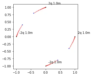
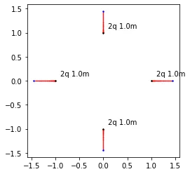
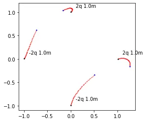
我正在尝试模拟一种粒子在电斥力（或吸引力）作用下飞向另一种粒子的现象，称为卢瑟福散射。我已经成功使用for循环和Python列表模拟了一些粒子。但是，现在我想使用numpy数组。该模型将采用以下步骤：

1. 对于所有粒子： 1. 计算与所有其他粒子的径向距离 2. 计算与所有其他粒子的夹角 3. 计算x方向和y方向的净力 2. 创建每个粒子的净xForce和yForce矩阵 3. 通过a = F / mass创建加速度（也是x和y分量）矩阵 4. 更新速度矩阵 5. 更新位置矩阵

我的问题是我不知道如何在计算力的分量时使用numpy数组。 以下是我的代码，但无法运行。

import numpy as np
# I used this function to calculate the force while using for-loops.
def force(x1, y1, x2, x2):
    angle =  math.atan((y2 - y1)/(x2 - x1))
    dr = ((x1-x2)**2 + (y1-y2)**2)**0.5
    force = charge2 * charge2 / dr**2 
    xforce = math.cos(angle) * force 
    yforce = math.sin(angle) * force

    # The direction of force depends on relative location
    if x1 > x2 and y1<y2:
        xforce = xforce
        yforce = yforce
    elif x1< x2 and y1< y2:
        xforce = -1 * xforce
        yforce = -1 * yforce
    elif x1 > x2 and y1 > y2:
        xforce = xforce
        yforce = yforce
    else:
        xforce = -1 * xforce
        yforce = -1* yforce

    return xforce, yforce

def update(array):

    # this for loop defeats the entire use of numpy arrays
    for particle in range(len(array[0])):
        # find distance of all particles pov from 1 particle

        # find all x-forces and y-forces on that particle

        xforce = # sum of all x-forces from all particles
        yforce = # sum of all y-forces from all particles
        force_arr[0, particle] = xforce
        force_arr[1, particle] = yforce

    return force

# begin parameters
t = 0
N = 3
masses = np.ones(N)
charges = np.ones(N)
loc_arr = np.random.rand(2, N)
speed_arr = np.random.rand(2, N)
acc_arr = np.random.rand(2, N)
force = np.random.rand(2, N)


while t < 0.5:
    force_arr = update(loc_arry)
    acc_arr = force_arr / masses
    speed_arr += acc_array
    loc_arr += speed_arr
    t += dt

    # plot animation

- Jelmer Mulder

---

这个 # this for loop defeats the entire use of numpy arrays 表示你想避免使用循环，但是想要进行“内联”计算？也许向量化是一个好的选择：https://towardsdatascience.com/python-vectorization-5b882eeef658 - L.Clarkson

Answer 1

一种使用数组对这个问题进行建模的方法可能是：

- 将点的坐标定义为一个 Nx2 数组。 (如果您以后要进阶到三维点，这将有助于扩展) - 将中间变量 distance, angle, force 定义为 NxN 数组，以表示成对交互。

关于 Numpy 的事情需要知道：

- 如果数组具有相同的形状（或符合形状，这是一个不容易的话题...），您可以在数组上调用大多数数字函数。 - meshgrid 可以帮助您生成计算 NxN 结果所需的数组索引，以便将您的 Nx2 数组转换形状。 - 一个正切的注意事项 arctan2() 计算一个有符号的角度，因此您可以避开复杂的 "哪个象限" 逻辑。

例如，您可以像这样做。请注意，在 get_dist 和 get_angle 中，两点之间的算术运算发生在最底层的维度中：

import numpy as np

# 2-D locations of particles
points = np.array([[1,0],[2,1],[2,2]])
N = len(points)  # 3

def get_dist(p1, p2):
    r = p2 - p1
    return np.sqrt(np.sum(r*r, axis=2))

def get_angle(p1, p2):
    r = p2 - p1
    return np.arctan2(r[:,:,1], r[:,:,0])

ii = np.arange(N)
ix, iy = np.meshgrid(ii, ii)

dist = get_dist(points[ix], points[iy])
angle = get_angle(points[ix], points[iy])
# ... compute force
# ... apply the force, etc.

对于上面所示的样本3点向量：

In [246]: dist
Out[246]: 
array([[0.        , 1.41421356, 2.23606798],
       [1.41421356, 0.        , 1.        ],
       [2.23606798, 1.        , 0.        ]])

In [247]: angle / np.pi     # divide by Pi to make the numbers recognizable
Out[247]: 
array([[ 0.        , -0.75      , -0.64758362],
       [ 0.25      ,  0.        , -0.5       ],
       [ 0.35241638,  0.5       ,  0.        ]])

- AbbeGijly

---

如果您知道您永远不需要超过2D，另一种方法是在复平面中建模点（x->Real，y->Imag），以保持您的点在一个漂亮紧凑的向量中。 - AbbeGijly

谢谢你的建议。我会确保在我的帖子中更新，一旦它能够正常工作。除了get_dist之外，我还可以使用distance.cdist(points, points)，这将给出完全相同的输出结果。由于这是任务的一部分，我可能会转向3D。 - Jelmer Mulder

Answer 2

以下是只使用循环进行每个时间步操作的示例，它适用于任意维度，我已经测试过3维：

from matplotlib import pyplot as plt
import numpy as np

fig, ax = plt.subplots()

N = 4
ndim = 2
masses = np.ones(N)
charges = np.array([-1, 1, -1, 1]) * 2
# loc_arr = np.random.rand(N, ndim)
loc_arr = np.array(((-1,0), (1,0), (0,-1), (0,1)), dtype=float)
speed_arr = np.zeros((N, ndim))

# compute charge matrix, ie c1 * c2
charge_matrix = -1 * np.outer(charges, charges)

time = np.linspace(0, 0.5)
dt = np.ediff1d(time).mean()

for i, t in enumerate(time):
    # get (dx, dy) for every point
    delta = (loc_arr.T[..., np.newaxis] - loc_arr.T[:, np.newaxis]).T
    # calculate Euclidean distance
    distances = np.linalg.norm(delta, axis=-1)
    # and normalised unit vector
    unit_vector = (delta.T / distances).T
    unit_vector[np.isnan(unit_vector)] = 0 # replace NaN values with 0

    # calculate force
    force = charge_matrix / distances**2 # norm gives length of delta vector
    force[np.isinf(force)] = 0 # NaN forces are 0

    # calculate acceleration in all dimensions
    acc = (unit_vector.T * force / masses).T.sum(axis=1)
    # v = a * dt
    speed_arr += acc * dt

    # increment position, xyz = v * dt
    loc_arr += speed_arr * dt 

    # plotting
    if not i:
        color = 'k'
        zorder = 3
        ms = 3
        for i, pt in enumerate(loc_arr):
            ax.text(*pt + 0.1, s='{}q {}m'.format(charges[i], masses[i]))
    elif i == len(time)-1:
        color = 'b'
        zroder = 3
        ms = 3
    else:
        color = 'r'
        zorder = 1
        ms = 1
    ax.plot(loc_arr[:,0], loc_arr[:,1], '.', color=color, ms=ms, zorder=zorder)

ax.set_aspect('equal')

上面的示例生成了以下图像，其中黑色和蓝色点分别表示起始和结束位置： 当电荷相等时charges = np.ones(N) * 2，系统对称性得以保持，电荷互相排斥： 最后，加入一些随机初始速度speed_arr = np.random.rand(N, 2)： 编辑

对上面的代码进行了小改动以确保其正确性。 （我漏掉了结果力上的-1，即+/+之间的力应为负数，而我在错误的轴上求和，对此深表歉意。现在，在masses[0] = 5的情况下，系统可以正确演化：

- Paddy Harrison

---

谢谢你的回答！如果我将质量改为不相等的值，似乎需要翻转质量列表才能使其正常工作。我遇到的另一个问题是，具有质量10 ** 99的粒子仍然会因来自质量为1的粒子的某些电力而移动相当多。 - Jelmer Mulder

你是对的！代码中有两个小错误，我已经纠正了它们，现在结果是一致的。我还添加了一个更大的质量示例。 - Paddy Harrison

非常感谢。我从来没有想到-1*和axis=1会解决它。 - Jelmer Mulder

Answer 3

传统的方法是计算系统中所有粒子的电场。假设您有三个带有正电荷的粒子：

particles = np.array([[1,0,0],[2,1,0],[2,2,0]]) # location of each particle
q = np.array([1,1,1]) # charge of each particle

计算每个粒子位置电场的最简单方法是使用循环：

def for_method(pos,q):
    """Computes electric field vectors for all particles using for-loop."""
    Evect = np.zeros( (len(pos),len(pos[0])) ) # define output electric field vector
    k =  1 / (4 * np.pi * const.epsilon_0) * np.ones((len(pos),len(pos[0]))) * 1.602e-19 # make this into matrix as matrix addition is faster
    # alternatively you can get rid of np.ones and just define this as a number
    
    for i, v0 in enumerate(pos): # s_p - selected particle | iterate over all particles | v0 reference particle
        for v, qc in zip(pos,q): # loop over all particles and calculate electric force sum | v particle being calculated for
            if all((v0 == v)):   # do not compute for the same particle
                continue
            else:
                r = v0 - v       #
                Evect[i] += r / np.linalg.norm(r) ** 3 * qc #! multiply by charge
    return Evect * k
# to find electric field at each particle`s location call
for_method(particles, q)

这个函数返回一个向量数组，形状与输入的particles数组相同。要找到每个粒子的力，只需将该向量与电荷数组q相乘即可。从那里开始，您可以轻松地找到加速度并使用您喜欢的ODE求解器集成系统。

性能优化和准确性

这种方法是可能最慢的方法。使用线性代数可以计算出场，从而获得显着的速度提升。以下代码是非常高效的Numpy矩阵“一行代码”（几乎是一行代码）来解决这个问题：

def CPU_matrix_method(pos,q):
    """Classic vectorization of for Coulomb law using numpy arrays."""
    k = 1 / (4 * np.pi * const.epsilon_0) * np.ones((len(pos),3)) * 1.602e-19 # define electric constant
    dist = distance.cdist(pos,pos)  # compute distances
    return k * np.sum( (( np.tile(pos,len(pos)).reshape((len(pos),len(pos),3)) - np.tile(pos,(len(pos),1,1))) * q.reshape(len(q),1)).T * np.power(dist,-3, where = dist != 0),axis = 1).T

请注意，以下代码还会返回每个粒子的电场向量。

如果你使用Cupy库将其转移到GPU上，您可以获得更高的性能。以下代码与CPU_matrix_method几乎相同，我只是稍微扩展了一行代码，以便您更好地了解正在发生的事情：

def GPU_matrix_method(pos,q):
    """GPU Coulomb law vectorization.
    Takes in numpy arrays, performs computations and returns cupy array"""
    # compute distance matrix between each particle
    k_cp = 1 / (4 * cp.pi * const.epsilon_0) * cp.ones((len(pos),3)) * 1.602e-19 # define electric constant, runs faster if this is matrix
    dist = cp.array(distance.cdist(pos,pos)) # could speed this up with cupy cdist function! use this: cupyx.scipy.spatial.distance.cdist
    pos, q = cp.array(pos), cp.array(q) # load inputs to GPU memory
    dist_mod = cp.power(dist,-3)        # compute inverse cube of distance
    dist_mod[dist_mod == cp.inf] = 0    # set all infinity entries to 0 (i.e. diagonal elements/ same particle-particle pairs)
    # compute by magic
    return k_cp * cp.sum((( cp.tile(pos,len(pos)).reshape((len(pos),len(pos),3)) - cp.tile(pos,(len(pos),1,1))) * q.reshape(len(q),1)).T * dist_mod, axis = 1).T

关于提到的算法的准确性，如果你在 particles 数组上计算这三种方法，你会得到相同的结果：

[[-6.37828367e-10 -7.66608512e-10  0.00000000e+00]
 [ 5.09048221e-10 -9.30757576e-10  0.00000000e+00]
 [ 1.28780145e-10  1.69736609e-09  0.00000000e+00]]

关于性能问题，我对每个算法进行了计算，系统范围从2到5000个带电粒子。此外，我还包括了 for_method 的Numba预编译版本，使for循环方法更具竞争力： 我们可以看到，for循环表现得非常糟糕，需要超过400秒才能计算出5000个粒子的系统。放大底部： 这表明，矩阵方法比这个问题的其他方法好了几个数量级。确切地说，5000个粒子的评估需要18.5秒的Numba for-loop，4秒的CPU矩阵（比Numba快5倍），以及0.8秒的GPU矩阵*（比Numba快23倍）。对于更大的数组，这种显着差异会更加明显。

* 使用的GPU是Nvidia K100。

- Jefeter_7