如何在ggplot中更改图例“Key”的方向？

Question

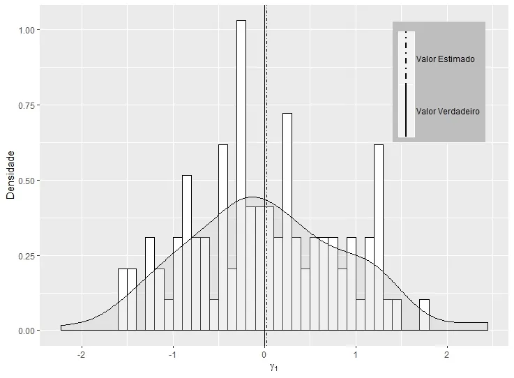
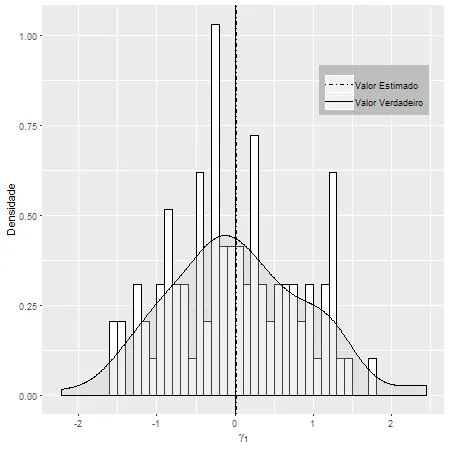
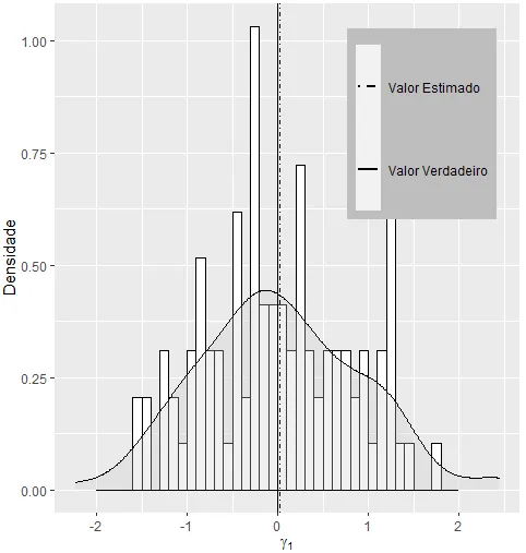
如何更改下面标题的键，使其水平而不改变图形的垂直线。

set.seed(000)
m <- matrix(rnorm(100,0,1),100,1)
dt <- data.frame(m)
names(dt) <- c("X")

library(ggplot2)

g2 <- ggplot(dt, aes(x=X)) 
g2 <- g2+geom_histogram(aes(y=..density..),      # Histogram with density instead of count on y-axis
                        binwidth=.5,
                        colour="black", fill="white",breaks=seq(-2, 2, by = 0.1)) 
g2 <- g2+geom_density(alpha=.3, fill="#cccccc") # Overlay with transparent density plot
g2 <- g2+  geom_vline(aes(xintercept=0, linetype="Valor Verdadeiro"),show.legend =TRUE)
g2 <- g2+  geom_vline(aes(xintercept=mean(dt$X, na.rm=T),    linetype="Valor Estimado"),show.legend =TRUE)
g2 <- g2+  scale_linetype_manual(values=c("dotdash","solid")) # Overlay with transparent density plot
g2 <- g2+  xlab(expression(paste(gamma[1])))+ylab("Densidade")
g2 <- g2+  theme(legend.key.height = unit(2, "cm") ,
                 legend.position = c(0.95, 0.95),
                 legend.justification = c("right", "top"),
                 legend.box.just = "right",
                 legend.margin = margin(6, 6, 6, 6),
                 legend.title=element_blank(),
                 legend.direction = "vertical",
                 legend.background = element_rect(fill="gray", size=.5, linetype="dotted"))
g2 <- g2+ guides(linetype = guide_legend(override.aes = list(size = 1)))
g2

注意：我想从位于 dotdash 和 solid 格式的标题内旋转线条。

请参考以下图片：

- fsbmat

---

您可能想要查看此解决方案： https://dev59.com/LJTfa4cB1Zd3GeqPS5Yb - Jeroen Boeye

@JeroenBoeye 它不起作用，我已经尝试过了！ - fsbmat

Answer 1

你可能需要使用 ggplot grob 并使用 grid 编辑函数来解决问题。

# Your data and plot
set.seed(000)
m <- matrix(rnorm(100,0,1),100,1)
dt <- data.frame(m)
names(dt) <- c("X")

library(ggplot2)

g2 <- ggplot(dt, aes(x=X)) 
g2 <- g2+geom_histogram(aes(y=..density..),      # Histogram with density instead of count on y-axis
                        binwidth=.5,
                        colour="black", fill="white",breaks=seq(-2, 2, by = 0.1)) 
g2 <- g2+geom_density(alpha=.3, fill="#cccccc") # Overlay with transparent density plot
g2 <- g2+  geom_vline(aes(xintercept=0, linetype="Valor Verdadeiro"),show.legend =TRUE)
g2 <- g2+  geom_vline(aes(xintercept=mean(dt$X, na.rm=T),    linetype="Valor Estimado"),show.legend =TRUE)
g2 <- g2+  scale_linetype_manual(values=c("dotdash","solid")) # Overlay with transparent density plot
g2 <- g2+  xlab(expression(paste(gamma[1])))+ylab("Densidade")
g2 <- g2+  theme(legend.key.height = unit(2, "cm") ,
                 legend.position = c(0.95, 0.95),
                 legend.justification = c("right", "top"),
                 legend.box.just = "right",
                 legend.margin = margin(6, 6, 6, 6),
                 legend.title=element_blank(),
                 legend.direction = "vertical",
                 legend.background = element_rect(fill="gray", size=.5, linetype="dotted"))
g2 <- g2+ guides(linetype = guide_legend(override.aes = list(size = 1)))


# Adjust key height and width
g2 = g2 + theme(
   legend.key.height = unit(.6, "cm"),
   legend.key.width = unit(1, "cm"))

# Get the ggplot Grob
  gt = ggplotGrob(g2)

# grid::grid.ls(grid.force(gt))  # To get a list of editable grobs

# Edit the relevant keys
library(grid)
 gt <- editGrob(grid.force(gt), gPath("key-[3,4]-1-[1,2]"), 
        grep = TRUE, global = TRUE,
        x0 = unit(0, "npc"), y0 = unit(0.5, "npc"), 
        x1 = unit(1, "npc"), y1 = unit(0.5, "npc")) 

# Draw it
grid.newpage()
grid.draw(gt)

- Sandy Muspratt

---

谢谢！有一个问题，如果我更改 legend.direction = "horizontal"，在您的代码中我应该在哪里更改以保持键水平？ - fsbmat

grid.ls(grid.force(gt) gives the list of editable grobs. With a horizontal legend, the relevant grobs begin with: key-1-3-1; key-1-3-2; key-1-7-1; key-1-7-2. Therefore, the gPath in the editGrob command will be: gPath("key-1-[3,7]-[1,2]") - Sandy Muspratt

非常感谢！你帮了我很多！ - fsbmat

我有同样的问题，但这段代码对我不起作用。 - iago

@iago 这段代码对我来说是有效的 - 对于这个例子。你能再具体一点吗？ - Sandy Muspratt

我找到了另一个解决方案。谢谢。 - iago

Answer 2

我发现这里，你现在可以在geom_vline调用中添加key_glyph：

library(ggplot2)
g2 <- ggplot(dt, aes(x=X)) 
g2 <- g2+geom_histogram(aes(y=..density..),      # Histogram with density instead of count on y-axis
                        binwidth=.5,
                        colour="black", fill="white",breaks=seq(-2, 2, by = 0.1)) 
g2 <- g2+geom_density(alpha=.3, fill="#cccccc") # Overlay with transparent density plot
g2 <- g2+  geom_vline(aes(xintercept=0, linetype="Valor Verdadeiro"),show.legend =TRUE, key_glyph = "path")
g2 <- g2+  geom_vline(aes(xintercept=mean(dt$X, na.rm=T),    linetype="Valor Estimado"),show.legend =TRUE, key_glyph = "path")
g2 <- g2+  scale_linetype_manual(values=c("dotdash","solid")) # Overlay with transparent density plot
g2 <- g2+  xlab(expression(paste(gamma[1])))+ylab("Densidade")
g2 <- g2+  theme(legend.key.height = unit(2, "cm") ,
                 legend.position = c(0.95, 0.95),
                 legend.justification = c("right", "top"),
                 legend.box.just = "right",
                 legend.margin = margin(6, 6, 6, 6),
                 legend.title=element_blank(),
                 legend.direction = "vertical",
                 legend.background = element_rect(fill="gray", size=.5, linetype="dotted"))
g2 <- g2+ guides(linetype = guide_legend(override.aes = list(size = 1)))
g2

- user63230