Pearson相关系数R和决定系数R平方是两个完全不同的统计量。
您可以参考以下网址:
https://en.wikipedia.org/wiki/Pearson_correlation_coefficient
和
https://en.wikipedia.org/wiki/Coefficient_of_determination
更新
Pearson相关系数r是衡量两个变量之间线性关系的统计量,其公式如下:

其中
bar x和
bar y分别为样本的均值。
而决定系数R2是衡量拟合优度的统计量,其公式如下:

其中
hat y为预测的
y值,
bar y为样本的均值。
因此,
- 它们衡量的是不同的东西
r**2不等于R2,因为它们的公式完全不同
更新2
只有在用线性模型计算变量(如
y)和预测变量
hat y的Pearson相关系数
r时,
r**2才等于
R2。
我们可以使用您提供的两个数组来进行示例演示。
import numpy as np
import pandas as pd
import scipy.stats as sps
import statsmodels.api as sm
from sklearn.metrics import r2_score as R2
import matplotlib.pyplot as plt
a = np.array([32.0, 25.97, 26.78, 35.85, 30.17, 29.87, 30.45, 31.93, 30.65, 35.49,
              28.3, 35.24, 35.98, 38.84, 27.97, 26.98, 25.98, 34.53, 40.39, 36.3])

b = np.array([28.778585, 31.164268, 24.690865, 33.523693, 29.272448, 28.39742,
              28.950092, 29.701189, 29.179174, 30.94298 , 26.05434 , 31.793175,
              30.382706, 32.135723, 28.018875, 25.659306, 27.232124, 28.295502,
              33.081223, 30.312504])
df = pd.DataFrame({
'x': a,
'y': b,
})
df.plot(x='x', y='y', marker='.', ls='none', legend=False);
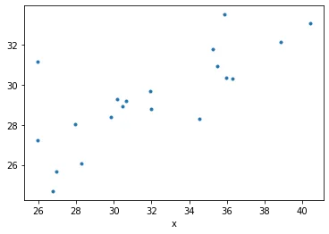
现在我们要拟合一个线性回归模型。
mod = sm.OLS.from_formula('y ~ x', data=df)
mod_fit = mod.fit()
print(mod_fit.summary())
输出
                            OLS Regression Results
==============================================================================
Dep. Variable:                      y   R-squared:                       0.580
Model:                            OLS   Adj. R-squared:                  0.557
Method:                 Least Squares   F-statistic:                     24.88
Date:                Mon, 29 Mar 2021   Prob (F-statistic):           9.53e-05
Time:                        14:12:15   Log-Likelihood:                -36.562
No. Observations:                  20   AIC:                             77.12
Df Residuals:                      18   BIC:                             79.12
Df Model:                           1
Covariance Type:            nonrobust
==============================================================================
                 coef    std err          t      P>|t|      [0.025      0.975]
------------------------------------------------------------------------------
Intercept     16.0814      2.689      5.979      0.000      10.431      21.732
x              0.4157      0.083      4.988      0.000       0.241       0.591
==============================================================================
Omnibus:                        6.882   Durbin-Watson:                   3.001
Prob(Omnibus):                  0.032   Jarque-Bera (JB):                4.363
Skew:                           0.872   Prob(JB):                        0.113
Kurtosis:                       4.481   Cond. No.                         245.
==============================================================================
计算r**2和R2,我们可以看到在这种情况下它们是相等的。
predicted_y = mod_fit.predict(df.x)
print("R2 :", R2(df.y, predicted_y))
print("r^2:", sps.pearsonr(df.y, predicted_y)[0]**2)
输出
R2 : 0.5801984323799696
r^2: 0.5801984323799696
你做的 R2(df.x, df.y) 不可能等于我们计算的值,因为你使用了一个独立的 x 和因变量 y 之间拟合程度的度量。相反,我们用 y 和预测值的 y,同时使用 r 和 R2。