更新: opts 已被弃用,请使用 theme 替代,如此答案所述。
为了更详细地解释kohske的答案,使下一个遇到这个问题的人更容易理解。
mtcars$cyl <- factor(mtcars$cyl, labels=c("four","six","eight"))
library(gridExtra)
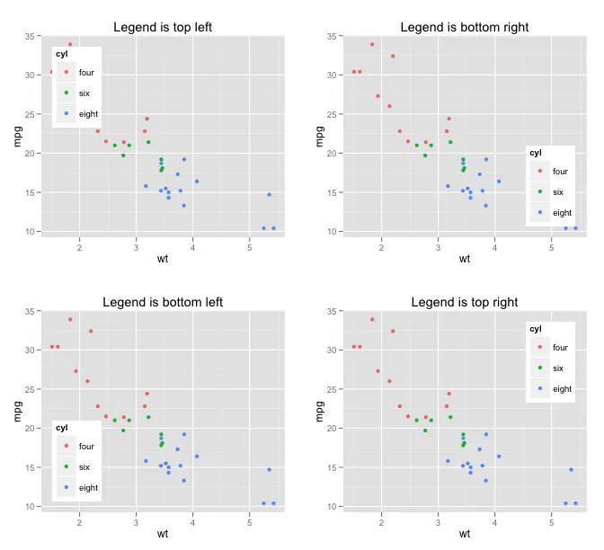
a <- ggplot(mtcars, aes(x=wt, y=mpg, colour=cyl)) + geom_point(aes(colour=cyl)) +
opts(legend.justification = c(0, 1), legend.position = c(0, 1), title="Legend is top left")
b <- ggplot(mtcars, aes(x=wt, y=mpg, colour=cyl)) + geom_point(aes(colour=cyl)) +
opts(legend.justification = c(1, 0), legend.position = c(1, 0), title="Legend is bottom right")
c <- ggplot(mtcars, aes(x=wt, y=mpg, colour=cyl)) + geom_point(aes(colour=cyl)) +
opts(legend.justification = c(0, 0), legend.position = c(0, 0), title="Legend is bottom left")
d <- ggplot(mtcars, aes(x=wt, y=mpg, colour=cyl)) + geom_point(aes(colour=cyl)) +
opts(legend.justification = c(1, 1), legend.position = c(1, 1), title="Legend is top right")
grid.arrange(a,b,c,d)
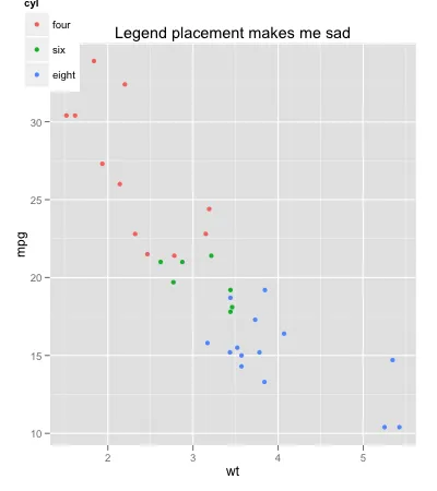
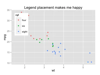
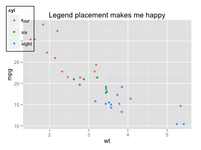
legend.position的正确坐标,以将图例放置在“数据区域”或灰色区域的角落。正如我在聊天中提到的那样,我怀疑像您这样的人可能需要权衡一下网格解决方案。 - joran