ggplot2:创建分面中的分面

4

我不知道我在标题中是否表达清楚了自己,但我希望当你看到下面的数字时,它是易于理解的。 首先,这是我的数据:

hydrocarbons    average SD  type    group
N   6,21    4,632774217 PAHs    Naphtalenes
N1  4,71    2,43670665  PAHs    Naphtalenes
N2  7,6 3,266286228 PAHs    Naphtalenes
N3  16,18   11,00643289 PAHs    Naphtalenes
N4  18,8    4,59631824  PAHs    Naphtalenes
F   16,87   7,022165062 PAHs    Fluorenes
F1  16,64   5,721267073 PAHs    Fluorenes
F2  18,67   8,467132345 PAHs    Fluorenes
F3  22,79   0,988021105 PAHs    Fluorenes
P   7,97    0,211647391 PAHs    Phenanthrenes
P1  26,66   16,64819987 PAHs    Phenanthrenes
P2  21,72   4,416811664 PAHs    Phenanthrenes
P3  18,99   4,635405486 PAHs    Phenanthrenes
P4  66,28   7,706085861 PAHs    Phenanthrenes
D   8,33    0,89862145  PAHs    Dibenzothiophenes
D1  8,63        PAHs    Dibenzothiophenes
D2  9,57        PAHs    Dibenzothiophenes
D3  20,69   3,453922632 PAHs    Dibenzothiophenes
D4  32,5    8,191613185 PAHs    Dibenzothiophenes
FL  10,37       PAHs    Fluoranthenes
PY  10,53       PAHs    Fluoranthenes
FL1 24,42   8,886055918 PAHs    Fluoranthenes
FL2 42,52   9,466539232 PAHs    Fluoranthenes
FL3 51,99   15,77786373 PAHs    Fluoranthenes
C   74,28   9,560499532 PAHs    Chrysenes
C1  46,56   15,86163409 PAHs    Chrysenes
C2  82,85   4,854714782 PAHs    Chrysenes
C3  114,42  41,70884318 PAHs    Chrysenes
nC-10   2,24        alkanes 
nC-11   2,24        alkanes 
nC-12   4,85    1,414267191 alkanes 
nC-13   5,54    0,089306765 alkanes 
nC-14   6,81    0,241222891 alkanes 
nC-15   5,56        alkanes 
nC-16   5,95        alkanes 
nC-17   5,82        alkanes 
nC-18   5,7     alkanes 
nC-19   6,41        alkanes 
nC-20   7,36        alkanes 
nC-21   6,24        alkanes 
nC-22   6,07        alkanes 
nC-23   6,35        alkanes 
nC-24   7,32        alkanes 
nC-25   6,6 2,215395794 alkanes 
nC-26   5,97    1,839829721 alkanes 
nC-27   6,51    1,972060107 alkanes 
nC-28   7,57    1,797509743 alkanes 
nC-29   8,37    3,004883333 alkanes 
nC-30   9,05    3,503601406 alkanes 
nC-31   10,27   4,242811665 alkanes 
nC-32   11,5    5,087821955 alkanes 
nC-33   14,31   8,085948386 alkanes 
nC-34   16,96   10,10105484 alkanes 
nC-35   20,52   14,1878649  alkanes 
nC-36   21,88   13,40071226 alkanes 
n-C5 (Pentane)  10,63   1,715015757 VOCs    
n-C6 (Hexane)   1,74    0,859880844 VOCs    
n-C7 (Heptane)  9,62    4,316473516 VOCs    
n-C9 (Nonane)   2,34    0,044641    VOCs    
Benzene 23,51   0,631882255 VOCs    
Toluene 18,48   2,369137637 VOCs    
Ethylbenzene    7,55    7,171631537 VOCs    
m-Xylene    12,53   7,250491275 VOCs    
p-Xylene    15,21   1,800247445 VOCs    
o-Xylene    21,96   2,184177383 VOCs    
Propylbenzene   12,8    15,31136895 VOCs    
n-Butylbenzene  9,33    5,486543125 VOCs    
n-Pentylbenzene 6,77    0,420247353 VOCs

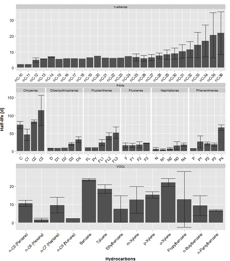
我想绘制我的碳氢化合物的“平均”半衰期,并根据“类型”进行分面。然而,只有对于“PAHs”类型,我希望按“组”进行附加分面。我能够编写和绘制的最佳代码是以下图像,但它并不完全符合我的要求:
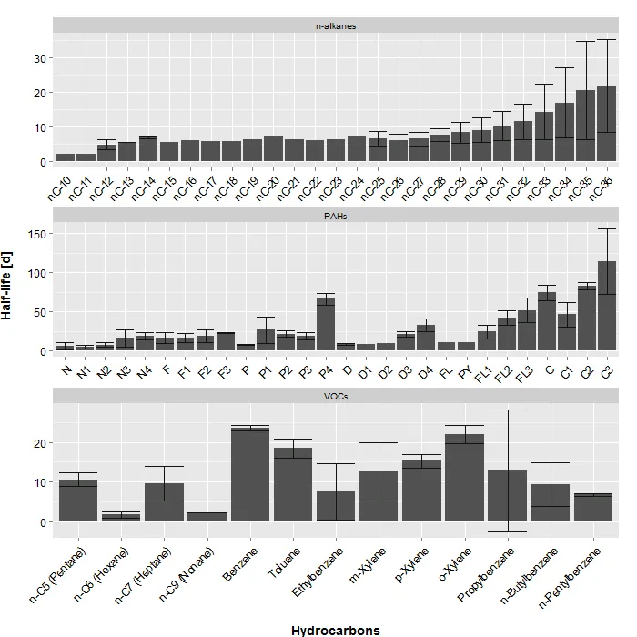
 hydrocarbon_halflifes 这是我正在使用的代码:
all <- read.delim2("E#6-results_chemistry.txt", header=TRUE)
library(ggplot2)
all$hydrocarbons <- factor(all$hydrocarbons, levels = all$hydrocarbons) #keeps the order of x-axis same as in table
levels(all$type)[levels(all$type)=="alkanes"] <- "n-alkanes" #if needed to change specific labels in a column
ggplot(all, aes(x=hydrocarbons, y=average)) +
  geom_bar(position = position_dodge(), stat="identity", fill="gray32") + 
  geom_errorbar(aes(ymin=average-SD, ymax=average+SD), color="gray8") + 
  facet_wrap(~type, scales="free", ncol=1) +
  ylab("Half-life [d]") + xlab("Hydrocarbons") +
  theme(axis.text.x=element_text(size=12, color="black", angle=45, hjust=1),
axis.title.x = element_text(size=14, face="bold", vjust=-0.7), 
axis.title.y = element_text(size=14, face="bold", vjust=2),
axis.text.y = element_text(size=12, colour="black"))

现在的问题是,是否可以制作一个图形,在现有的一个中添加一个额外的面部条,仅针对“PAHs”类型,根据“组”进行分组?图形可能看起来像这样: facet_in_facet 
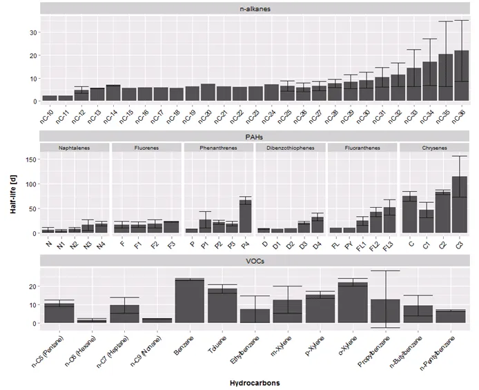
如果可能的话,对于“PAHs”,我也可以制作第二个x轴,根据“组”进行排列。
谢谢, Deni
1个回答

5
我认为你需要深入了解ggplot结构。这种方法采用原始图形,但去掉中间面板(但保留空间)。我将中间面板作为一个单独的图形进行构建,并包括“PAHs”级别的外观。我从该图形中提取相关材料(绘图面板、条纹、x轴和y轴),并将其插入到原始图形的空白处。然后,我构建了一个新条纹来包含变量名“PAHs”。该方法确保三个面板的高度相同,unit(1,"null")。(在下面的图表之后,请参见我使用的all数据框。)

小修改:更新到ggplot2 2.2.1

library(ggplot2)
library(gtable)
library(grid)
all$hydrocarbons <- factor(all$hydrocarbons, levels = all$hydrocarbons) #keeps the order of x-axis same as in table
   levels(all$type)[levels(all$type)=="alkanes"] <- "n-alkanes" #if needed to change specific labels in a column

# Original plot
pAll <- ggplot(all, aes(x = hydrocarbons, y = average)) +
  geom_bar(position = position_dodge(), stat="identity", fill = "gray32") + 
  geom_errorbar(aes(ymin = average-SD, ymax = average+SD), color = "gray8") + 
  facet_wrap( ~ type, scales = "free", ncol = 1) +
  ylab("Half-life [d]") + xlab("Hydrocarbons") +
  theme(axis.text.x = element_text(size = 12, color = "black", angle = 45, hjust = 1),
     axis.title.x = element_text(size = 14, face = "bold", vjust = -0.7), 
     axis.title.y = element_text(size = 14, face = "bold", vjust = 2),
     axis.text.y = element_text(size = 12, colour = "black"))

# Middle plot, but with facets for 'PAHs'
pMid <- ggplot(subset(all, type == "PAHs"), aes(x = hydrocarbons, y = average)) +
  geom_bar(position = position_dodge(), stat = "identity", fill = "gray32") + 
  geom_errorbar(aes(ymin = average - SD, ymax = average + SD), color = "gray8") + 
  facet_grid(. ~ group, scales = "free", space = "free") +
  ylab("Half-life [d]") + 
  theme(axis.text.x = element_text(size = 12, color = "black", angle = 45, hjust = 1),
     axis.title.x = element_text(size = 14, face = "bold", vjust = -0.7), 
     axis.title.y = element_text(size = 14, face = "bold", vjust = 2),
     axis.text.y = element_text(size = 12, colour = "black"))

# Get the ggplot grobs
gAll <- ggplotGrob(pAll)
gMid <- ggplotGrob(pMid)

# In gMid, get the positions of the panels in the layout: t = top, l = left, ...
pos1 <- c(subset(gMid$layout, grepl("panel", gMid$layout$name), select = t:r))

# Extract 'panels' (along with x-axis and strips)
panels <- gMid[(unique(pos1$t) - 1) : (unique(pos1$t) + 1), min(pos1$l) : max(pos1$l)]
# Extract 'axisL' - y-axis
axisL <- gMid[unique(pos1$t), min(pos1$l) - 1]

# In gAll, get the positions of the panel of the middle plot in the layout
pos2 <- c(subset(gAll$layout, grepl("panel", gAll$layout$name), select = t:r))
pos2 <- lapply(pos2, "[", 2)

# Drop original panel material in the middle plot
drop <- gAll$layout$name %in% c("panel-1-2", "strip-t-1-2", "axis-b-1-2", "axis-l-2-1")
gAll$grobs[drop] <- NULL
gAll$layout <- gAll$layout[!drop,]

# Add new 'panels' to gAll
gAll <- gtable_add_grob(gAll, panels, t = pos2$t-1, l = pos2$l, b = pos2$t+1,  name = "panels")

# Add new 'axisL' to gAll
gAll <- gtable_add_grob(gAll, axisL, t = pos2$t, l = pos2$l-1, name = "strips")

# Add row above the current strips
gAll <- gtable_add_rows(gAll, gAll$heights[pos2$t-1], pos2$t-2)  

# Add grob, a new strip containing variable name 'PAHs', into the new row
gAll <- gtable_add_grob(gAll, 
  list(rectGrob(gp = gpar(col = NA, fill = "gray85")),
       textGrob("PAHs", gp = gpar(fontsize = 9.6))), 
  t = pos2$t-1, l = pos2$l, name = c("background", "text"))

# Add a small gap between the strips
gAll <- gtable_add_rows(gAll, unit(1/10, "line"), pos2$t-1)

# Probably not needed, but if axisB font size in pMid is different from pAll
gAll$heights[pos2$t + 3] <- gMid$heights[unique(pos1$t) + 1]

# Draw it
grid.newpage()
grid.draw(gAll)

enter image description here


all = structure(list(hydrocarbons = structure(c(21L, 28L, 29L, 30L, 
31L, 12L, 13L, 14L, 15L, 60L, 62L, 63L, 64L, 65L, 6L, 7L, 8L, 
9L, 10L, 16L, 67L, 17L, 18L, 19L, 2L, 3L, 4L, 5L, 32L, 33L, 34L, 
35L, 36L, 37L, 38L, 39L, 40L, 41L, 42L, 43L, 44L, 45L, 46L, 47L, 
48L, 49L, 50L, 51L, 52L, 53L, 54L, 55L, 56L, 57L, 58L, 23L, 24L, 
25L, 26L, 1L, 68L, 11L, 20L, 61L, 59L, 66L, 22L, 27L), .Label = c("Benzene", 
"C", "C1", "C2", "C3", "D", "D1", "D2", "D3", "D4", "Ethylbenzene", 
"F", "F1", "F2", "F3", "FL", "FL1", "FL2", "FL3", "m-Xylene", 
"N", "n-Butylbenzene", "n-C5 (Pentane)", "n-C6 (Hexane)", "n-C7 (Heptane)", 
"n-C9 (Nonane)", "n-Pentylbenzene", "N1", "N2", "N3", "N4", "nC-10", 
"nC-11", "nC-12", "nC-13", "nC-14", "nC-15", "nC-16", "nC-17", 
"nC-18", "nC-19", "nC-20", "nC-21", "nC-22", "nC-23", "nC-24", 
"nC-25", "nC-26", "nC-27", "nC-28", "nC-29", "nC-30", "nC-31", 
"nC-32", "nC-33", "nC-34", "nC-35", "nC-36", "o-Xylene", "P", 
"p-Xylene", "P1", "P2", "P3", "P4", "Propylbenzene", "PY", "Toluene"
), class = "factor"), average = c(6.21, 4.71, 7.6, 16.18, 18.8, 
16.87, 16.64, 18.67, 22.79, 7.97, 26.66, 21.72, 18.99, 66.28, 
8.33, 8.63, 9.57, 20.69, 32.5, 10.37, 10.53, 24.42, 42.52, 51.99, 
74.28, 46.56, 82.85, 114.42, 2.24, 2.24, 4.85, 5.54, 6.81, 5.56, 
5.95, 5.82, 5.7, 6.41, 7.36, 6.24, 6.07, 6.35, 7.32, 6.6, 5.97, 
6.51, 7.57, 8.37, 9.05, 10.27, 11.5, 14.31, 16.96, 20.52, 21.88, 
10.63, 1.74, 9.62, 2.34, 23.51, 18.48, 7.55, 12.53, 15.21, 21.96, 
12.8, 9.33, 6.77), SD = c(4.632774217, 2.43670665, 3.266286228, 
11.00643289, 4.59631824, 7.022165062, 5.721267073, 8.467132345, 
0.988021105, 0.211647391, 16.64819987, 4.416811664, 4.635405486, 
7.706085861, 0.89862145, NA, NA, 3.453922632, 8.191613185, NA, 
NA, 8.886055918, 9.466539232, 15.77786373, 9.560499532, 15.86163409, 
4.854714782, 41.70884318, NA, NA, 1.414267191, 0.089306765, 0.241222891, 
NA, NA, NA, NA, NA, NA, NA, NA, NA, NA, 2.215395794, 1.839829721, 
1.972060107, 1.797509743, 3.004883333, 3.503601406, 4.242811665, 
5.087821955, 8.085948386, 10.10105484, 14.1878649, 13.40071226, 
1.715015757, 0.859880844, 4.316473516, 0.044641, 0.631882255, 
2.369137637, 7.171631537, 7.250491275, 1.800247445, 2.184177383, 
15.31136895, 5.486543125, 0.420247353), type = structure(c(2L, 
2L, 2L, 2L, 2L, 2L, 2L, 2L, 2L, 2L, 2L, 2L, 2L, 2L, 2L, 2L, 2L, 
2L, 2L, 2L, 2L, 2L, 2L, 2L, 2L, 2L, 2L, 2L, 1L, 1L, 1L, 1L, 1L, 
1L, 1L, 1L, 1L, 1L, 1L, 1L, 1L, 1L, 1L, 1L, 1L, 1L, 1L, 1L, 1L, 
1L, 1L, 1L, 1L, 1L, 1L, 3L, 3L, 3L, 3L, 3L, 3L, 3L, 3L, 3L, 3L, 
3L, 3L, 3L), .Label = c("alkanes", "PAHs", "VOCs"), class = "factor"), 
    group = structure(c(6L, 6L, 6L, 6L, 6L, 5L, 5L, 5L, 5L, 7L, 
    7L, 7L, 7L, 7L, 3L, 3L, 3L, 3L, 3L, 4L, 4L, 4L, 4L, 4L, 2L, 
    2L, 2L, 2L, 1L, 1L, 1L, 1L, 1L, 1L, 1L, 1L, 1L, 1L, 1L, 1L, 
    1L, 1L, 1L, 1L, 1L, 1L, 1L, 1L, 1L, 1L, 1L, 1L, 1L, 1L, 1L, 
    1L, 1L, 1L, 1L, 1L, 1L, 1L, 1L, 1L, 1L, 1L, 1L, 1L), .Label = c("", 
    "Chrysenes", "Dibenzothiophenes", "Fluoranthenes", "Fluorenes", 
    "Naphtalenes", "Phenanthrenes"), class = "factor")), .Names = c("hydrocarbons", 
"average", "SD", "type", "group"), class = "data.frame", row.names = c(NA, 
-68L))

非常感谢 @SandyMuspratt!! 这个完美地解决了我的问题,正是我想要的。只有一个小注释,在创建带有PAHs分面的中间图时,我添加了一行额外的代码来保持我想要的组的顺序: "all$group <- factor(all$group, levels = c("Naphtalenes","Fluorenes","Phenanthrenes","Dibenzothiophenes","Fluoranthenes","Chrysenes")) #将x轴的顺序与表格中相同" - Deni Galinac Ribičić

网页内容由stack overflow 提供, 点击上面的
可以查看英文原文,
原文链接