3个回答
3
R wikibook 中有一些关于 R 产出质量的好资料。
我认为这个函数来自 Paul Johnson,它在 wikibook 中列出,正是你所需要的。
我认为这个函数来自 Paul Johnson,它在 wikibook 中列出,正是你所需要的。
http://pj.freefaculty.org/R/WorkingExamples/outreg-worked.R
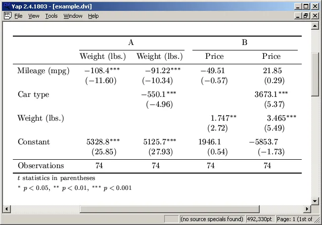
我编辑了这个函数以适应booktabs格式,并允许有额外属性的模型:
- chandler
3
您可能需要使用'memisc'包中的
mtable函数。它有关联的LaTeX输出参数:==========================================================================
Model 1 Model 2 Model 3
--------------------------------------------------------------------------
Constant 30.628*** 6.360*** 28.566***
(7.409) (1.252) (7.355)
Percentage of population under 15 -0.471** -0.461**
(0.147) (0.145)
Percentage of population over 75 -1.934 -1.691
(1.041) (1.084)
Real per-capita disposable income 0.001 -0.000
(0.001) (0.001)
Growth rate of real per-capita disp. income 0.529* 0.410*
(0.210) (0.196)
--------------------------------------------------------------------------
sigma 3.931 4.189 3.803
R-squared 0.262 0.162 0.338
F 8.332 4.528 5.756
p 0.001 0.016 0.001
N 50 50 50
==========================================================================
这是您得到的LaTeX代码:
texfile123 <- "mtable123.tex"
write.mtable(mtable123,forLaTeX=TRUE,file=texfile123)
file.show(texfile123)
#------------------------
%%%%%%%%%%%%%%%%%%%%%%%%%%%%%%%%%%%%%%%%%%%%%%%%%%%%%%%%%%%%%%%%%%%%%%%%%%%%%%%%%%%%%%%%%%%%%%%
%
% Calls:
% Model 1:  lm(formula = sr ~ pop15 + pop75, data = LifeCycleSavings)
% Model 2:  lm(formula = sr ~ dpi + ddpi, data = LifeCycleSavings)
% Model 3:  lm(formula = sr ~ pop15 + pop75 + dpi + ddpi, data = LifeCycleSavings)
%
%%%%%%%%%%%%%%%%%%%%%%%%%%%%%%%%%%%%%%%%%%%%%%%%%%%%%%%%%%%%%%%%%%%%%%%%%%%%%%%%%%%%%%%%%%%%%%%
\begin{tabular}{lcD{.}{.}{7}cD{.}{.}{7}cD{.}{.}{7}}
\toprule
&&\multicolumn{1}{c}{Model 1} && \multicolumn{1}{c}{Model 2} && \multicolumn{1}{c}{Model 3}\\
\midrule
Constant                                    &  & 30.628^{***} &&  6.360^{***} && 28.566^{***}\\
                                            &  &  (7.409)     &&  (1.252)     &&  (7.355)    \\
Percentage of population under 15           &  & -0.471^{**}  &&              && -0.461^{**} \\
                                            &  &  (0.147)     &&              &&  (0.145)    \\
Percentage of population over 75            &  &  -1.934      &&              &&  -1.691     \\
                                            &  &  (1.041)     &&              &&  (1.084)    \\
Real per-capita disposable income           &  &              &&   0.001      &&  -0.000     \\
                                            &  &              &&  (0.001)     &&  (0.001)    \\
Growth rate of real per-capita disp. income &  &              &&  0.529^{*}   &&  0.410^{*}  \\
                                            &  &              &&  (0.210)     &&  (0.196)    \\
\midrule
sigma                                       &  &     3.931    &&     4.189    &&     3.803   \\
R-squared                                   &  &     0.262    &&     0.162    &&     0.338   \\
F                                           &  &     8.332    &&     4.528    &&     5.756   \\
p                                           &  &     0.001    &&     0.016    &&     0.001   \\
N                                           &  &    50        &&    50        &&    50       \\
\bottomrule
\end{tabular}
- IRTFM
1
xtable 可以做到这一点,但有点像黑客。
取两个线性模型,命名为 lm.x 和 lm.y。
如果您使用以下代码:
myregtables <- rbind(xtable(summary(lm.x)), xtable(summary(lm.y)))
xtable 将生成一个包含两个回归模型的表格。 如果在 LaTeX 中添加 \hline(或者可能是两个),那么它应该看起来不错。 您仍然只有一个标签和标题用于这两个模型。 正如我所说,这是一个有点像黑客的解决方案。
- richiemorrisroe
2
谢谢,里奇。由于这是一种相对常见的呈现数据的方式,我认为一定有更简单的方法来完成它。 - Rafael Magalhães
1@RafaelMagalhães,编写代码并不难(我最近查看了xtable的内部结构,它们非常清晰)。但这不是我会使用的东西,所以可能需要其他人来完成。 - richiemorrisroe
网页内容由stack overflow 提供, 点击上面的可以查看英文原文,
原文链接
原文链接
xtable嵌套模型的方法。现在我可以发布图片了,希望我的目标会更清晰;@ Chase 和 @ joran,非常感谢你们的帮助。现在我需要想办法嵌套这些模型。@ Spacedman,我没有特定的期刊,只是一篇学期论文。我也在使用Latex,并希望找到一个将表格直接导出到Latex的函数,而不是手动组装模型系数。 - Rafael Magalhães