不同大小的多个ggplot图表

Question

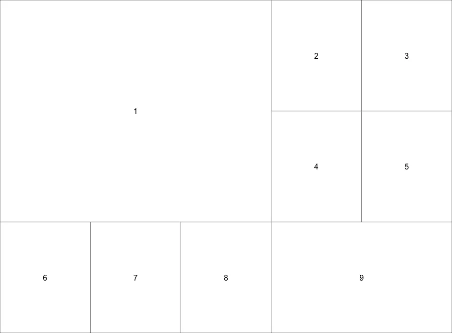
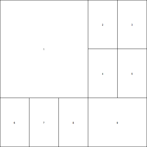
使用gridExtra包中的grid.arrange可以相对简单地将多个绘图排列成矩阵，但是当一些绘图要比其他绘图大时，该如何排列绘图（我正在使用的是ggplot2）？ 在基础设施中，我可以使用layout()，如下面的示例：

 nf <- layout(matrix(c(1,1,1,2,3,1,1,1,4,5,6,7,8,9,9), byrow=TRUE, nrow=3))
 layout.show(nf)

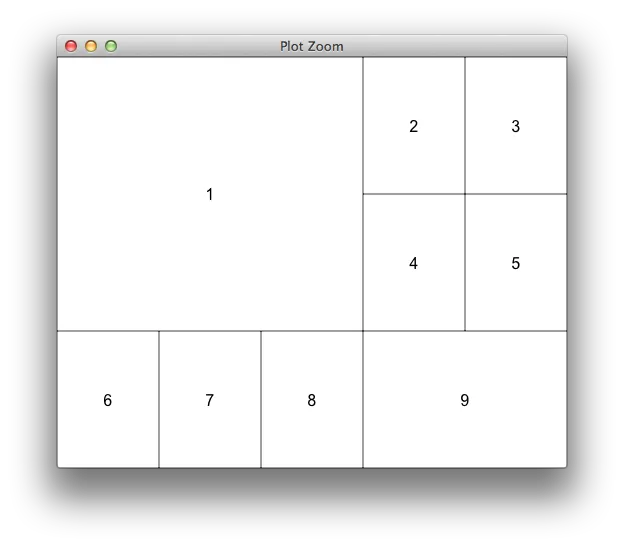
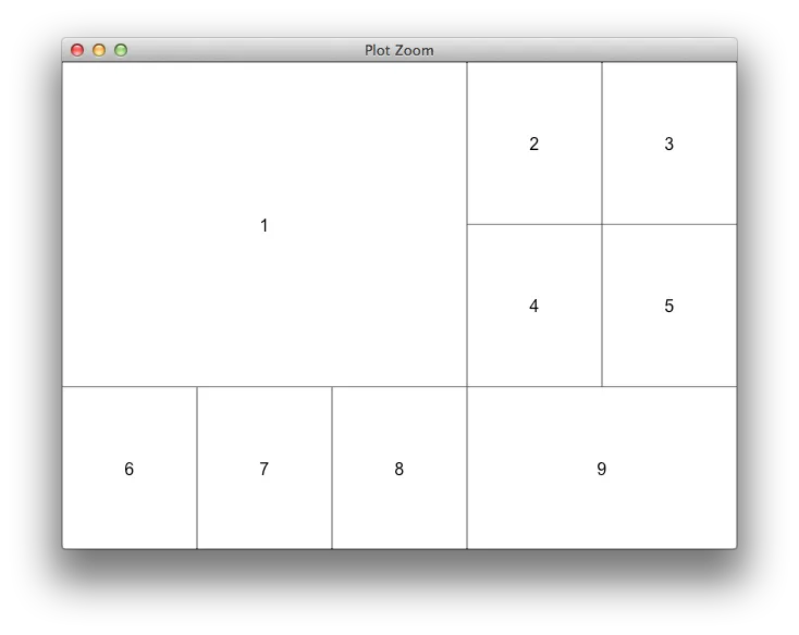
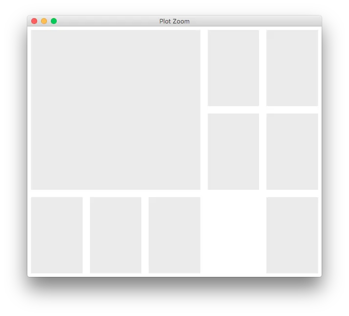
ggplot图形的等价物是什么？

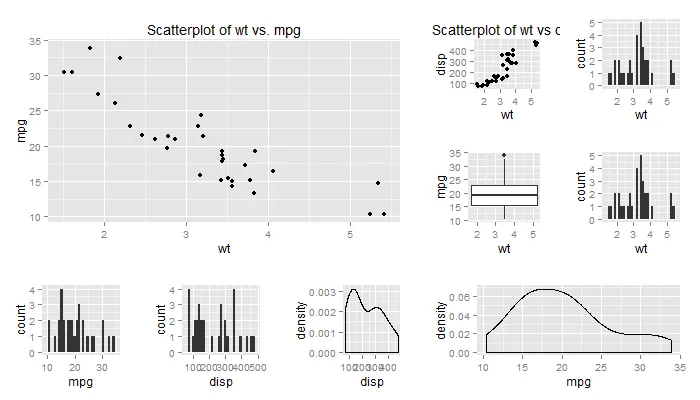
一些可供包含的图形

library(ggplot2)
p1 <- qplot(x=wt,y=mpg,geom="point",main="Scatterplot of wt vs. mpg", data=mtcars)
p2 <- qplot(x=wt,y=disp,geom="point",main="Scatterplot of wt vs disp", data=mtcars)
p3 <- qplot(wt,data=mtcars)
p4 <- qplot(wt,mpg,data=mtcars,geom="boxplot")
p5 <- qplot(wt,data=mtcars)
p6 <- qplot(mpg,data=mtcars)
p7 <- qplot(disp,data=mtcars)
p8 <- qplot(disp, y=..density.., geom="density", data=mtcars)
p9 <- qplot(mpg, y=..density.., geom="density", data=mtcars)

- Hugh

---

这个SO问题可能会有所帮助。 - Didzis Elferts

Answer 1

你可以像这个例子一样使用嵌套的arrangeGrob调用：

library(ggplot2)
library(gridExtra)

p <- ggplot(data.frame(x=1, y=1), aes(x,y)) + geom_point()

grid.arrange(
  arrangeGrob(
    p, 
    arrangeGrob(p, p, nrow=2),
    ncol=2 ,widths=c(2,1)),
  arrangeGrob(p, p ,p ,ncol=3, widths=rep(1,3)),
  nrow=2)

编辑：

gl <- lapply(1:9, function(ii) grobTree(rectGrob(),textGrob(ii)))

grid.arrange(
  arrangeGrob(gl[[1]],
              do.call(arrangeGrob, c(gl[2:5], ncol=2)),
              nrow=1,
              widths=3:2),
  do.call(arrangeGrob, c(gl[6:9], nrow=1, list(widths=c(1,1,1,2)))),
nrow=2, heights=c(2,1))

- Roland

---

在使用do.call时不需要匿名函数，因为arrangeGrob的定义中已经包含了...。 - baptiste

@baptiste 我知道并使用 nrow，但是当尝试传递 widths 时出现了错误。 - Roland

这是因为c()函数在处理列表时的工作方式。需要使用do.call(arrangeGrob, c(gl[6:9], nrow=1, list(widths=c(1,1,1,2))))。 - baptiste

Answer 2

使用gtable的替代方案

（注：此处可能需要根据上下文稍作调整）

library(gtable)

gl <- lapply(1:9, function(ii) grobTree(textGrob(ii), rectGrob()))
# gl <- lapply(1:9, function(ii) ggplotGrob(qplot(1,1) + ggtitle(ii)))

gt <- gtable(widths=unit(rep(1,5), "null"),
             heights=unit(rep(1,3), "null"))

gtable_add_grobs <- gtable_add_grob # alias

gt <- gtable_add_grobs(gt, gl, 
                       l=c(1,4,5,4,5,1,2,3,4),
                       r=c(3,4,5,4,5,1,2,3,5),
                       t=c(1,1,1,2,2,3,3,3,3),
                       b=c(2,1,1,2,2,3,3,3,3))
grid.newpage()
grid.draw(gt)

- baptiste

---

这似乎是一种流行的方法，但我无法弄清楚如何将类似于ggplot的grobs添加到图中。（在Roland的示例中，这很容易。）你能解释一下如何添加绘图吗？（我在OP中包含了一些示例图。） - Hugh

ggplotGrob 将 ggplot 转换为 grob，在我的示例中有一行注释使用它。 - baptiste

Answer 3

你可以使用与布局相同的矩阵界面来使用grid.arrange。

library(gridExtra)
library(grid)
gl <- lapply(1:9, function(ii) grobTree(rectGrob(), textGrob(ii)))

grid.arrange(grobs = gl, layout_matrix = rbind(c(1,1,1,2,3),
                                               c(1,1,1,4,5),
                                               c(6,7,8,9,9)))

同样的方法也适用于ggplots; 注意，NA可以用来表示空白单元格。结果是一个gtable，与ggsave()兼容。

gl <- replicate(9, ggplot(), FALSE)
grid.arrange(grobs = gl, layout_matrix = rbind(c(1,1,1,2,3),
                                               c(1,1,1,4,5),
                                               c(6,7,8,NA,9)))

- baptiste

Answer 4

我非常感谢其他回答，但Didzis Elferts的评论与我发现最容易实现的答案相关联。

library(ggplot2)
p1 <- qplot(x=wt,y=mpg,geom="point",main="Scatterplot of wt vs. mpg", data=mtcars)
p2 <- qplot(x=wt,y=disp,geom="point",main="Scatterplot of wt vs disp", data=mtcars)
p3 <- qplot(wt,data=mtcars)
p4 <- qplot(wt,mpg,data=mtcars,geom="boxplot")
p5 <- qplot(wt,data=mtcars)
p6 <- qplot(mpg,data=mtcars)
p7 <- qplot(disp,data=mtcars)
p8 <- qplot(disp, y=..density.., geom="density", data=mtcars)
p9 <- qplot(mpg, y=..density.., geom="density", data=mtcars)

vplayout <- function(x, y) viewport(layout.pos.row = x, layout.pos.col = y)

grid.newpage()
pushViewport(viewport(layout = grid.layout(3, 5))) # 3 rows, 5 columns
print(p1, vp = vplayout(1:2, 1:3))  # the big plot covers rows 1:2 and cols 1:3
print(p2, vp = vplayout(1, 4))
print(p3, vp = vplayout(1, 5))
print(p4, vp = vplayout(2, 4))
print(p5, vp = vplayout(2, 5))
print(p6, vp = vplayout(3, 1))
print(p7, vp = vplayout(3, 2))
print(p8, vp = vplayout(3, 3))
print(p9, vp = vplayout(3, 4:5))

- Hugh

---

太好了！有没有办法在超级图的顶部添加一个单独的标题？ - Pertinax

Answer 5

我喜欢由lay_out函数提供的界面（以前在wq包中）。它采用list(plot, row(s), column(s))形式的参数。以下是一个示例：

lay_out(list(p1, 1:2, 1:3),
       list(p2, 1, 4),
       list(p3, 1, 5),
       list(p4, 2, 4),
       list(p5, 2, 5),
       list(p6, 3, 1),
       list(p7, 3, 2),
       list(p8, 3, 3),
       list(p9, 3, 4:5))

产生的结果如下：

lay_out = function(...) {    
    x <- list(...)
    n <- max(sapply(x, function(x) max(x[[2]])))
    p <- max(sapply(x, function(x) max(x[[3]])))
    grid::pushViewport(grid::viewport(layout = grid::grid.layout(n, p)))    

    for (i in seq_len(length(x))) {
        print(x[[i]][[1]], vp = grid::viewport(layout.pos.row = x[[i]][[2]], 
            layout.pos.col = x[[i]][[3]]))
    }
} 

这段代码来源于较早版本的wq包，可以在非官方Github CRAN镜像的提交历史中找到。

- Gregor Thomas

---

这是最简单的解决方案，但似乎layOut函数不再存在。您是否知道其他直接的选项？ - Meli

谢谢。有没有办法让它可以将ggplot和非ggplot图形结合起来使用？ - Meli

它应该适用于任何“网格”图形，这主要意味着“ggplot”和“lattice”。如果您想使用“base”图形，则可以尝试使用“gridBase”包。 - Gregor Thomas