如何在R中为散点图中的类别添加颜色？

Question

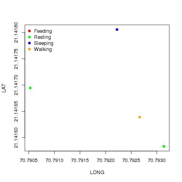
我有一些以csv格式存储的数据。我想将这些数据绘制成不同颜色的图表，以4种不同的活动为基准，每种活动对应一种颜色。

ACTIVITY     LAT            LONG
Resting   21.14169444   70.79052778
Feeding   21.14158333   70.79313889
Resting   21.14158333   70.79313889
Walking   21.14163889   70.79266667
Walking   21.14180556   70.79222222
Sleeping  21.14180556   70.79222222

我已尝试以下代码，但它没有起作用：

ACTIVITY.cols <- cut(ACTIVITY, 5, labels = c("pink", "green", "yellow","red","blue"))
plot(Data$Latitude,Data$Longitude, col = as.character(ACTIVITY.cols)

并且

plot(Data$Latitude,Data$Longitude, col=c("red","blue","green","yellow")[Data$ACTIVITY]

- user4993868

Answer 1

使用

txt <- "ACTIVITY     LAT            LONG
Resting   21.14169444   70.79052778
Feeding   21.14158333   70.79313889
Resting   21.14158333   70.79313889
Walking   21.14163889   70.79266667
Walking   21.14180556   70.79222222
Sleeping  21.14180556   70.79222222"
dat <- read.table(text = txt, header = TRUE)

一种选择是使用ACTIVITY变量作为索引，从长度为nlevels(ACTIVITY)的颜色向量中进行索引。

cols <- c("red","green","blue","orange")
plot(LAT ~ LONG, data = dat, col = cols[dat$ACTIVITY], pch = 19)
legend("topleft", legend = levels(dat$ACTIVITY), col = cols, pch = 19, bty = "n")

这将产生： 为了看到这为什么可行，cols被扩展为：

> cols[dat$ACTIVITY]
[2] "green"  "red"    "green"  "orange" "orange" "blue"

因为ACTIVITY是一个因素，但以数字1,2,...,n的形式存储。

其他更高级的解决方案也可用，考虑使用ggplot2包来简单创建相同的绘图。

library("ggplot2")
plt <- ggplot(dat, aes(x = LONG, y = LAT, colour = ACTIVITY)) +
  geom_point()
plt

这将会产生以下结果：

- Gavin Simpson

---

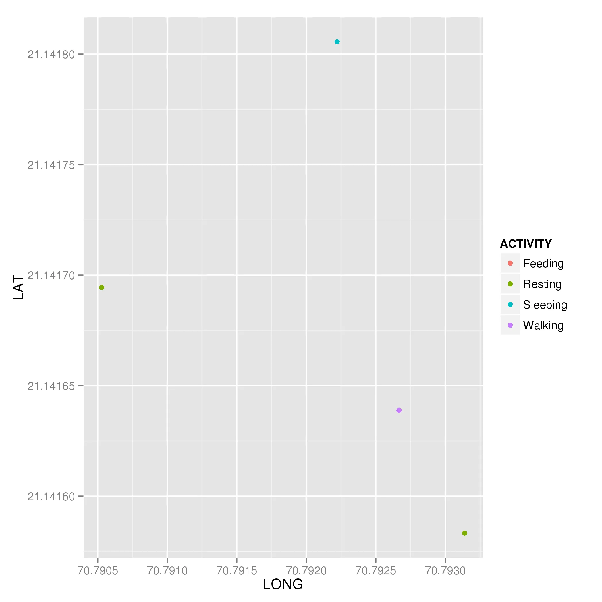
如果您熟悉基本绘图系统，并想要一些 ggplot2 的功能，qplot 函数可以为您提供基本功能，其语法更接近于基本绘图的常规风格。 - tegancp

@tegancp 我从来不喜欢 qplot()，而且我认为在第二版的GGplot书中，Hadley正在淡化 qplot() 的作用。 - Gavin Simpson

我认为一般情况下可以避免使用qplot()，一旦你理解了ggplot2的操作方式。然而，对于那些已经使用过R的plot()（或类似工具）但可能会因陌生的术语和语法而感到不安的人来说，它作为使用ggplot()的垫脚石还是有价值的。 - tegancp

жИСзЬЯзЪДиЃ§дЄЇеЬ®е≠¶дє†ggplot()зїШеЫЊеЈ•дљЬжЧґпЉМеЃГдЉЪ嶮зҐНжИСдїђзЪДињЫеЇ¶гАВ - Gavin Simpson

Answer 2

使用ggplot2包，它更快且更美观。

library(ggplot2)
ggplot("your dataframe") + geom_point(aes(x = Latitude, y = Longitude, colour = factor(ACTIVITY)))

- Mostafa90

Answer 3

这里是我如何使用命名向量定义颜色的方法：

set.seed(1);
N <- 30;
df <- data.frame(activity=sample(c('Resting','Feeding','Walking','Sleeping'),N,replace=T),lat=runif(N,0,100),long=runif(N,0,100));
cols <- c(Resting='red',Feeding='blue',Walking='green',Sleeping='yellow');
par(mar=c(5,4,4,6)+0.1,xaxs='i',yaxs='i');
plot(df$lat,df$long,xlim=c(0,100),ylim=c(0,100),col=cols[as.character(df$activity)],main='Activity Locations',xlab='Latitude',ylab='Longitude');
legend(103,80,names(cols),col=cols,pch=1,xpd=T);

- bgoldst