如何在R中计算非线性最小二乘的置信区间？

Question

我在使用R中的nls函数预测置信区间时遇到了一些问题。

pl <- ggplot(data) +  geom_point(aes(x=date, y=cases),size=2, colour="black") + xlab("Date") + ylab("Cases")  
model = nls(cases ~ SSlogis(log(date), Asym, xmid, scal), data= data )


new.data = data.frame(date=c(1:100))
interval <- predict(model, newdata = new.data, se.fit = TRUE, interval = "confidence", level= 0.9)

new.data[c("fit","lwr.conf", "upr.conf")] <- interval 

pl +   
  geom_ribbon(data=new.data, aes(x=date, ymin=lwr.pred, ymax=upr.pred), alpha=0.05, inherit.aes=F, fill="blue")

当我运行它时，没有错误显示，但我获得的间隔只是一个包含适合值的向量，而不是上下置信区间。

- A Jorg

---

你能否发布一些样本数据？请编辑问题并附上dput(data)的输出结果。如果太大，请附上dput(head(data, 20))的输出结果。 - Rui Barradas

predict.nls 的文档对参数 se.fit 说道: "目前该参数被忽略。" - Rui Barradas

是的，我知道，我只是为了以防万一放置它。 - A Jorg

Answer 1

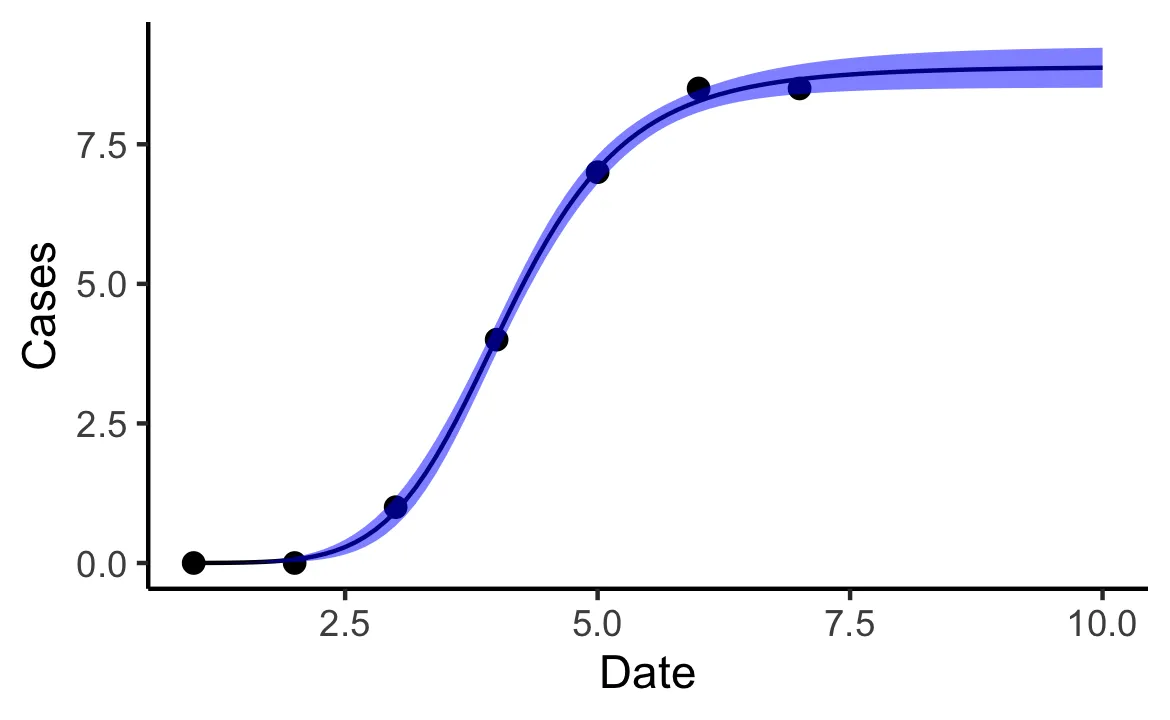
我知道3种方法可以做到这一点，其中一种在其他答案中有描述。以下是其他选项。第一种使用nls()来拟合模型，investr::predFit用于进行预测和CI：

 library(tidyverse)
 library(investr)
 data <- tibble(date = 1:7,
                cases = c(0, 0, 1, 4, 7, 8.5, 8.5))

    model <- nls(cases ~ SSlogis(log(date), Asym, xmid, scal), data= data )
    new.data <- data.frame(date=seq(1, 10, by = 0.1))
    interval <- as_tibble(predFit(model, newdata = new.data, interval = "confidence", level= 0.9)) %>% 
      mutate(date = new.data$date)

    p1 <- ggplot(data) +  geom_point(aes(x=date, y=cases),size=2, colour="black") + xlab("Date") + ylab("Cases")  

    p1+
      geom_line(data=interval, aes(x = date, y = fit ))+
      geom_ribbon(data=interval, aes(x=date, ymin=lwr, ymax=upr), alpha=0.5, inherit.aes=F, fill="blue")+
      theme_classic()

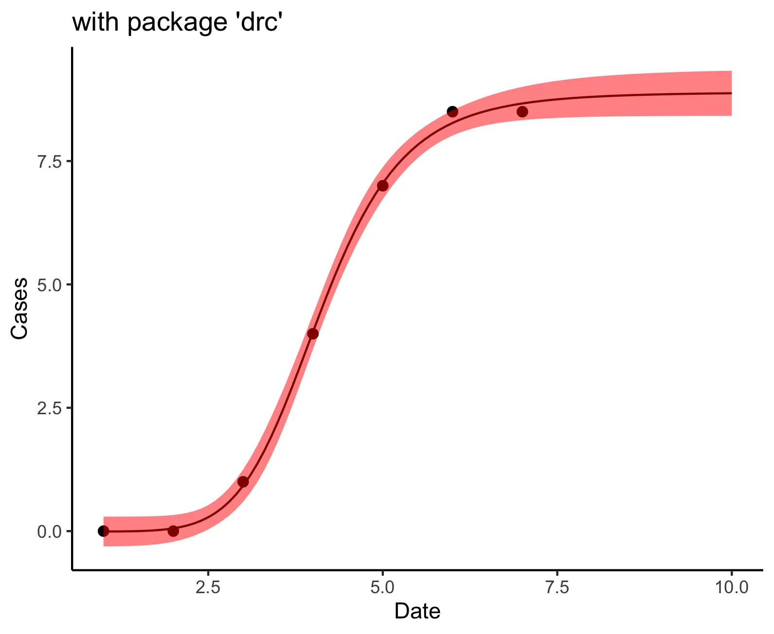
另一个选择是使用“drc” 包进行模型拟合和预测（也称为剂量-反应曲线）。该包使用内置的启动器函数（需要使用或创建），但 “drc” 类对象具有许多有用的方法，其中一个是支持置信区间的 predict.drc 方法（尽管仅适用于某些内置的自启动器）。以下是使用“drc” 包的示例：

library(drc)
model_drc <- drm(cases~date, data = data, fct=LL.4())
predict_drc <- as_tibble(predict(model_drc, newdata = new.data, interval = "confidence", level = 0.9)) %>% 
  mutate(date = new.data$date)

p1+
  geom_line(data=predict_drc, aes(x = date, y = Prediction ))+
  geom_ribbon(data=predict_drc, aes(x=date, ymin=Lower, ymax=Upper), alpha=0.5, inherit.aes=F, fill="red")+
  ggtitle("with package 'drc'")+
  theme_classic()

关于'drc'包的更多信息：期刊论文，博客文章描述自定义自启动的drc，以及文档。

- bs93

Answer 2

使用propagate包进行模拟，可以获得非线性置信区间：

library("propagate")

x  <- c(25, 25, 10, 10, 5, 5, 2.5, 2.5, 1.25, 1.25)
y <- c(0.0998, 0.0948, 0.076, 0.0724, 0.0557,
       0.0575, 0.0399, 0.0381, 0.017, 0.0253)

m <- nls(y ~ SSmicmen(x, Vm, K), trace = TRUE)

x1 <- seq(0, 25, length = 100)
plot(x, y, xlim = c(0, 25), ylim = c(0, 0.1))
lines(x1, predict(m, data.frame(S = x1)), col = "red")

y.conf <- predictNLS(m, newdata=data.frame(x=x1), interval="confidence", alpha=0.05, nsim=10000)$summary
y.pred <- predictNLS(m, newdata=data.frame(x=x1), interval="prediction", alpha=0.05, nsim=10000)$summary

matlines(x1, y.conf[,c("Sim.2.5%", "Sim.97.5%")], col="red", lty="dashed")
matlines(x1, y.pred[,c("Sim.2.5%", "Sim.97.5%")], col="blue", lty="solid")

- tpetzoldt