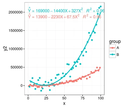
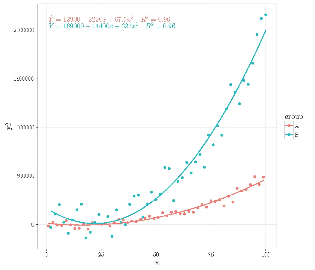
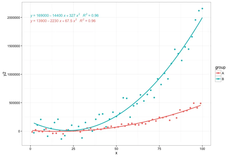
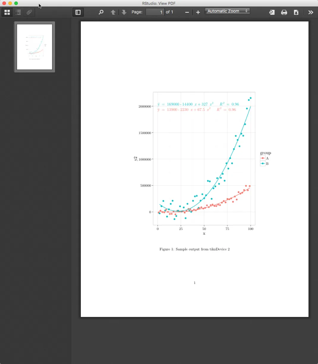
在ggpmisc中使用`round`或`sprintf`函数对回归方程进行格式化，`dev="tikz"`。

Question

在ggpmisc中使用`round`或`sprintf`函数对回归方程进行格式化，`dev="tikz"`。

4

我可以使用round或sprintf函数来控制回归方程中的数字显示吗？我还不知道如何在使用eq.with.lhs = "hat(Y)~=~"时使用dev="tikz".

library(ggplot2)
library(ggpmisc)

# generate artificial data
set.seed(4321)
x <- 1:100
y <- (x + x^2 + x^3) + rnorm(length(x), mean = 0, sd = mean(x^3) / 4)
my.data <- data.frame(x, 
                      y, 
                      group = c("A", "B"), 
                      y2 = y * c(0.5,2),
                      block = c("a", "a", "b", "b"))

str(my.data)

# plot
ggplot(data = my.data, mapping=aes(x = x, y = y2, colour = group)) +
        geom_point() +
        geom_smooth(method = "lm", se =  FALSE, formula = y ~ poly(x=x, degree = 2, raw = TRUE)) +
        stat_poly_eq(
                       mapping     = aes(label = paste(..eq.label.., ..rr.label.., sep = "~~~"))
                     , data        = NULL
                     , geom        = "text"
                     , formula     = y ~ poly(x, 2, raw = TRUE)
                     , eq.with.lhs = "hat(Y)~`=`~"
                     , eq.x.rhs    = "X"
                     , label.x     = 0
                     , label.y     = 2e6
                     , vjust       = c(1.2, 0)
                     , position    = "identity"
                     , na.rm       = FALSE
                     , show.legend = FALSE
                     , inherit.aes = TRUE
                     , parse       = TRUE
                     ) +
        theme_bw()

- MYaseen208

round和sprintf之间有一个重要的区别。第一个根据数学规则对值进行四舍五入，而第二个仅根据指定的结构截取数字。我更喜欢sprintf，因为它是一种打印值的方法。 - FlorianSchunke

你说的舍入是什么意思？是指系数的物理舍入（例如，将67.5舍入为68），还是调整函数使其更接近插入函数（减去噪声）？前者是一个编程问题，而后者则更多地涉及数学性质。每个问题只提出一个问题也更清晰（对于dev=tikz的问题很容易创建一个独立的最小工作示例）。否则，您可能会遇到仅想接受两个答案的情况，因为它们各自回答了一个部分。 - takje

1

关于一个问题包含两个问题的观点非常好。无论如何，我现在的答案回答了两个问题。round和signif返回数字值，sprintf返回字符值。根据格式规范，sprintf将使用与round或signif等效的方式来转换数字。 - Pedro J. Aphalo

2个回答

1

Myaseen208，

以下是解决使用 ggpmisc::stat_poly_eq() 创建 .tex 输出问题的解决方法。我确认您目前无法将 stat_poly_eq() 和 "hat(Y)~=~" 与 library(tikzDevice) 结合使用来创建latex .tex 输出。然而，我已经提供了一种解决方案，在过渡期间可以创建正确的 .tex 输出。

ggpmisc 包的创建者 Pedro Aphalo 已经非常友善地接受了对 ggpmisc::stat_poly_eq() 的增强请求。请参考下面提交的错误报告。

代码示例：

以下代码将生成一个没有帽子符号的图形：

# Load required packages
requiredPackages <- requiredPackages <- c("ggplot2", "ggpmisc", "tikzDevice", "latex2exp")

# ipak - Check to see if the package is installed, if not install and then load...
ipak <- function(pkg)
{
  new.pkg <- pkg[!(pkg %in% installed.packages()[, "Package"])]
  if (length(new.pkg))
    install.packages(new.pkg, dependencies = TRUE)
  sapply(pkg, require, character.only = TRUE)
}

ipak(requiredPackages)

# generate artificial data
set.seed(4321)
x <- 1:100
y <- (x + x ^ 2 + x ^ 3) + rnorm(length(x), mean = 0, sd = mean(x ^ 3) / 4)
my.data <- data.frame(
  x, y,
  group = c("A", "B"),
  y2 = y * c(0.5, 2),
  block = c("a", "a", "b", "b")
)

# Define Formaula..
formulaDefined <- (y ~ (poly(x = x, degree = 2, raw = TRUE)))

gp <- ggplot(data = my.data, mapping = aes(x = x, y = y2, colour = group))
gp <- gp + geom_point()
gp <- gp + geom_smooth(method = "lm", se =  FALSE, formula = formulaDefined )
gp <- gp + stat_poly_eq(
  aes(label = paste(..eq.label.., "~~~", ..rr.label.., sep = "")),
#  eq.with.lhs = "italic(hat(y))~`=`~",
  formula     = formulaDefined,
  geom        = "text",
  label.x     = 0,
  label.y     = 2e6,
  vjust       = c(1.2, 0),
  position    = "identity",
  na.rm       = FALSE,
  show.legend = FALSE,
  inherit.aes = TRUE,
  parse       = TRUE)
gp <- gp + theme_bw()
gp

我们现在可以修改这段代码及其 tikz输出，以创建所需的结果：

Tikz 代码解决方案

第一步是修改代码以输出所需的 .tex 文件。完成后，我们可以利用 gsub() 在 .tex 文件中找到需要的行，并将 {\itshape y}; 替换为 {\^{y}}; [第646和693行]。

# Load required packages
requiredPackages <- requiredPackages <- c("ggplot2", "ggpmisc", "tikzDevice", "latex2exp")

# ipak - Check to see if the package is installed, if not install and then load...
ipak <- function(pkg)
{
  new.pkg <- pkg[!(pkg %in% installed.packages()[, "Package"])]
  if (length(new.pkg))
    install.packages(new.pkg, dependencies = TRUE)
  sapply(pkg, require, character.only = TRUE)
}

ipak(requiredPackages)

# generate artificial data
set.seed(4321)
x <- 1:100
y <- (x + x ^ 2 + x ^ 3) + rnorm(length(x), mean = 0, sd = mean(x ^ 3) / 4)
my.data <- data.frame(
  x, y,
  group = c("A", "B"),
  y2 = y * c(0.5, 2),
  block = c("a", "a", "b", "b")
)

setwd("~/dev/stackoverflow/37242863")

texFile <- "./test2.tex"
# setup tex output file
tikz(file = texFile, width = 5.5, height = 5.5)

#Define Formaula..
formulaDefined <- (y ~ (poly(x = x, degree = 2, raw = TRUE)))

gp <- ggplot(data = my.data, mapping = aes(x = x, y = y2, colour = group))
gp <- gp + geom_point()
gp <- gp + geom_smooth(method = "lm", se =  FALSE, formula = formulaDefined )
gp <- gp + stat_poly_eq(
  aes(label = paste(..eq.label.., "~~~", ..rr.label.., sep = "")),
#  eq.with.lhs = "italic(hat(y))~`=`~",
  formula     = formulaDefined,
  geom        = "text",
  label.x     = 0,
  label.y     = 2e6,
  vjust       = c(1.2, 0),
  position    = "identity",
  na.rm       = FALSE,
  show.legend = FALSE,
  inherit.aes = TRUE,
  parse       = TRUE)
gp <- gp + theme_bw()
gp
dev.off()

## OK, now we can take the test.txt file and replace the relevant attributes to
## add the hat back to the y in the .tex output file...

texOutputFile <- readLines(texFile)
y <- gsub('itshape y', '^{y}', texOutputFile )
cat(y, file=texFile, sep="\n")

Tex测试框架：

为了测试解决方案，我们可以创建一个小的LaTeX测试工具。您可以在RStudio [t1.tex]中加载此文件，然后编译它；它将引入通过先前呈现的代码生成的test2.text。

注意：RStudio是从R编译的LaTeX输出的绝佳平台。

\documentclass{article}

\usepackage{tikz}

\begin{document}

\begin{figure}[ht]
\input{test2.tex}
\caption{Sample output from tikzDevice 2}
\end{figure}

\end{document}

结果：

替代方案

另一个选择可能是使用geom_text()，这种方法的缺点是您必须自己编写回归线方程函数。这在您之前的帖子中已经讨论过：在图表上添加回归线方程和R2

如果您需要详细的解决方案[使用geom_text]，那么请联系我。另一个选择是向ggpmisc提交错误报告[我已完成]，看看作者是否已经解决或可以解决。

错误报告：https://bitbucket.org/aphalo/ggpmisc/issues/1/stat_poly_eq-fails-when-used-with

希望以上内容能帮到您。

- Technophobe01

@pedro-aphalo 有没有更好的方法使用 ggpmisc？ - Technophobe01

2

我会在下一个版本中调查这个问题。我认为需要输出有效的LaTeX代码而不是R表达式。因为昨天我提交了ggpmisc 0.2.8到CRAN，今天早上已经被接受，所以需要几周时间。我有LaTeX的经验，所以很容易做到。 - Pedro J. Aphalo

1

Pedro，感谢您的快速回复。非常感谢您的帮助。保重。目前这个解决方案应该可以让@MYaseen208继续进行。 - Technophobe01

网页内容由stack overflow 提供, 点击上面的

可以查看英文原文，
原文链接

- Pedro J. Aphalo · Accepted Answer

1）如果使用“ggpmisc”（版本>=0.2.9），下面的代码将回答问题中的dev="tikz"部分。

\documentclass{article}

\begin{document}

<<setup, include=FALSE, cache=FALSE>>=
library(knitr)
opts_chunk$set(fig.path = 'figure/pos-', fig.align = 'center', fig.show = 'hold',
               fig.width = 7, fig.height = 6, size = "footnotesize", dev="tikz")
@


<<>>=
library(ggplot2)
library(ggpmisc)
@

<<>>=
# generate artificial data
set.seed(4321)
x <- 1:100
y <- (x + x^2 + x^3) + rnorm(length(x), mean = 0, sd = mean(x^3) / 4)
my.data <- data.frame(x,
                      y,
                      group = c("A", "B"),
                      y2 = y * c(0.5,2),
                      block = c("a", "a", "b", "b"))

str(my.data)
@

<<>>=
# plot
ggplot(data = my.data, mapping=aes(x = x, y = y2, colour = group)) +
  geom_point() +
  geom_smooth(method = "lm", se =  FALSE, 
              formula = y ~ poly(x=x, degree = 2, raw = TRUE)) +
  stat_poly_eq(
    mapping     = aes(label = paste("$", ..eq.label.., "$\\ \\ \\ $",
                       ..rr.label.., "$", sep = ""))
    , geom        = "text"
    , formula     = y ~ poly(x, 2, raw = TRUE)
    , eq.with.lhs = "\\hat{Y} = "
    , output.type = "LaTeX"
   ) +
  theme_bw()
@

\end{document}

感谢您提出这个增强功能，我自己也一定会找到它的用途！

2）回答问题中关于round和sprintf的部分。您不能使用round或sprintf来更改数字的位数，stat_poly_eq目前使用三个有效数字的signif作为整个系数向量的参数。如果您想要完全控制，则可以使用另一个统计数据，即stat_fit_glance，它也在ggpmisc（>= 0.2.8）中，它在内部使用broom:glance。它更加灵活，但您将不得不在aes调用内部自行处理所有格式，目前有一个注意事项，broom::glance似乎不能正确地与poly配合使用，您需要明确编写多项式方程以作为传递给formula的参数。