ggplot2：在极坐标系下用直线连接点

Question

coord_polar会使线条呈现出极坐标系，但有时你可能不想这样做（例如当空间被认为是离散而不是连续的时候）：

iris %>% gather(dim, val, -Species) %>%
  group_by(dim, Species) %>% summarise(val = mean(val)) %>% 
  ggplot(aes(dim, val, group=Species, col=Species)) + 
    geom_line(size=2) + coord_polar()

之前的解决方法不再有效。有没有什么新的解决办法？

- geotheory

---

嗯，对于连续轴我同意，但对于部分离散空间并不一定如此。在这里，ggplot似乎强制执行了实际上应该是美学选择的内容。 - geotheory

"ggradar" 可能有用，然而... - geotheory

并不完全是这样。它是在数据点之间插值一个等间距序列，就像在笛卡尔空间中一样。要在极坐标空间中绘制直线，需要一个变化的斜率。然而，更大的问题是：无论坐标空间如何，对于非有序分类数据的线图都会产生误导。 - alistaire

所以你的意思是平行坐标图本质上是具有误导性的吗？（我特别喜欢维基百科页面上用的那个例子的讽刺意味...） - geotheory

我并不是在说它们是饼图（饼图也有维基百科文章），但某种程度上，由于人们阅读从左到右的图表的本能（至少对于LTR语言的母语者来说），这一点是正确的。与平行坐标轴相结合，即使轴顺序任意，也可能暗示因果关系。然而，它们仍然可以用于视觉聚类，而且交互性（能够切换轴顺序、选择等）可以极大地改善它们的效果。 - alistaire

@alistaire 不确定饼图的相关性 - 我的例子是一个径向平行坐标图。我在一般意义上欣赏你的观点，但在平行坐标方面不太认同。许多图形方法会“误导”一些不那么有文化素养的读者 - 这并不否定它们的价值或有效性 :) - geotheory

Answer 1

在极坐标下，用直线连接数据点的图形也被称为雷达图。

Erwan Le Pennec撰写了一篇名为“从平行坐标到雷达图”的文章，介绍如何使用ggplot2创建雷达图。他建议使用coord_radar()函数来定义。文章链接：From Parallel Plot to Radar Plot。

coord_radar <- function (theta = "x", start = 0, direction = 1) {
  theta <- match.arg(theta, c("x", "y"))
  r <- if (theta == "x") "y" else "x"
  ggproto("CordRadar", CoordPolar, theta = theta, r = r, start = start, 
          direction = sign(direction),
          is_linear = function(coord) TRUE)
}

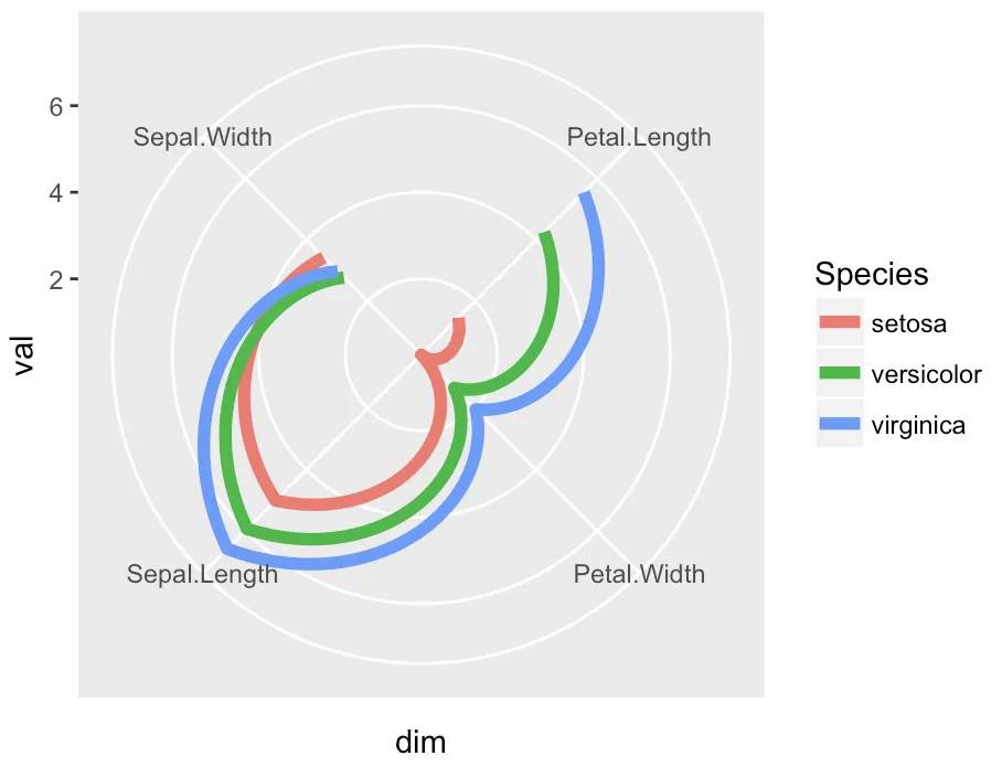
通过这个，我们可以创建如下的图表：

library(tidyr)
library(dplyr)
library(ggplot2)

iris %>% gather(dim, val, -Species) %>%
  group_by(dim, Species) %>% summarise(val = mean(val)) %>% 
  ggplot(aes(dim, val, group=Species, col=Species)) + 
  geom_line(size=2) + coord_radar()

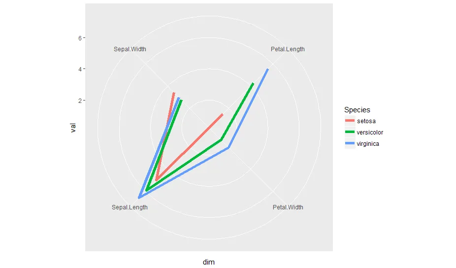
coord_radar() 是 ggiraphExtra 包的一部分。因此，您可以直接使用它。

iris %>% gather(dim, val, -Species) %>%
      group_by(dim, Species) %>% summarise(val = mean(val)) %>% 
      ggplot(aes(dim, val, group=Species, col=Species)) + 
      geom_line(size=2) + ggiraphExtra:::coord_radar()

请注意，coord_radar()函数不被该软件包导出。因此，需要使用三个冒号（:::）来访问该函数。

- Uwe

---

顶级答案！你有参与 ggiraphExtra 的开发吗？ - geotheory

@geotheory，我很高兴找到了解决方案。不，我与 ggiraphExtra 无关。首先，我在谷歌上搜索“straight lines coord_polar”，找到了 Erwan Le Pennec 的论文，在其中给予 Hadley Wickham 对 coord_radar() 的认可。然后，我试图找到 Hadley 的参考资料，但最终只得到了 RDocumentation 上 ggiraphExtra 包中 coord_radar() 的链接。 - Uwe

刚刚注意到 geom_polygon 不需要这个解决方法。但是对于线条/路径仍然非常必要。 - geotheory

哎呀，忘记勾选这个了！ - geotheory

但是会在vline和hline方面出现问题。 - Saren Tasciyan