Gnuplot: 散点图和密度图

Question

我有一些表示星团的x和y数据点。我想使用Gnuplot和它的散点函数来可视化密度，包括重叠点。

我使用了以下命令：

 set style fill transparent solid 0.04 noborder
 set style circle radius 0.01
 plot "data.dat" u 1:2 with circles lc rgb "red"

结果如下：

结果：

但我想要这样的效果

Gnuplot有这种可能吗？ 有什么想法吗？

- Gilfoyle

Answer 1

(编辑：修订并简化)

可能比我的之前的回答更好的方法是：

对于每个数据点，请检查在半径为R内有多少其他数据点。您需要调整R的值以获得一些合理的图形。

索引数据行需要gnuplot>=5.2.0和一个没有空行的数据块。您可以先将文件绘制到数据块中（请检查help table）或者参见这里： gnuplot: load datafile 1:1 into datablock

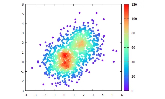
创建此图表所需的时间将随着数据点数量的增加而增加，O(N^2)，因为您必须检查每个点与所有其他点的关系。我不确定是否有更聪明、更快的方法。下面的示例具有1200个数据点，将在我的笔记本电脑上花费约4秒钟。您基本上可以应用相同的原则用于3D。

脚本: 适用于gnuplot>=5.2.0

### 2D density color plot
reset session

t1 = time(0.0)
# create some random rest data
set table $Data
    set samples 700
    plot '+' u (invnorm(rand(0))):(invnorm(rand(0))) w table
    set samples 500
    plot '+' u (invnorm(rand(0))+2):(invnorm(rand(0))+2) w table
unset table
print sprintf("Time data creation: %.3f s",(t0=t1,t1=time(0.0),t1-t0))

# for each datapoint: how many other datapoints are within radius R
R = 0.5     # Radius to check
Dist(x0,y0,x1,y1) = sqrt((x1-x0)**2 + (y1-y0)**2)
set print $Density
    do for [i=1:|$Data|] {
        x0 = real(word($Data[i],1))
        y0 = real(word($Data[i],2))
        c  = 0
        stats $Data u (Dist(x0,y0,$1,$2)<=R ? c=c+1 : 0) nooutput
        d = c / (pi * R**2)             # density: points per unit area
        print sprintf("%g %g %d", x0, y0, d)
    }
set print
print sprintf("Time density check: %.3f sec",(t0=t1,t1=time(0.0),t1-t0))

set size ratio -1   # same screen units for x and y
set palette rgb 33,13,10
plot $Density u 1:2:3 w p pt 7 lc palette z notitle
### end of script

结果:

（注：该内容为一个html代码段，翻译后仍需保留html格式）

- theozh

Answer 2

尽管这个问题已经比较“老”，问题可能已经以不同的方式解决了……这可能更多是出于好奇和乐趣而非实际目的。以下代码仅使用gnuplot实现了根据点密度进行着色的功能。在我的旧电脑上，绘制1000个点需要几分钟时间。我很想知道是否可以改进此代码，特别是在速度方面（不使用外部工具）。遗憾的是，gnuplot没有提供基本功能，如排序、查找表、合并、转置或其他基本函数（我知道……它是gnuplot……而不是分析工具）。

代码:

### density color plot 2D
reset session

# create some dummy datablock with some distribution
N = 1000
set table $Data
    set samples N
    plot '+' u (invnorm(rand(0))):(invnorm(rand(0))) w table
unset table
# end creating dummy data

stats $Data u 1:2 nooutput
XMin = STATS_min_x
XMax = STATS_max_x
YMin = STATS_min_y
YMax = STATS_max_y
XRange = XMax-XMin
YRange = YMax-YMin
XBinCount = 20
YBinCount = 20
BinNo(x,y) = floor((y-YMin)/YRange*YBinCount)*XBinCount + floor((x-XMin)/XRange*XBinCount)

# do the binning
set table $Bins
    plot $Data u (BinNo($1,$2)):(1) smooth freq # with table
unset table

# prepare final data: BinNo, Sum, XPos, YPos
set print $FinalData
do for [i=0:N-1] {
    set table $Data3
    plot $Data u (BinNumber = BinNo($1,$2),$1):(XPos = $1,$1):(YPos = $2,$2) every ::i::i with table
    plot [BinNumber:BinNumber+0.1] $Bins u (BinNumber == $1 ? (PointsInBin = $2,$2) : NaN) with table
    print sprintf("%g\t%g\t%g\t%g", XPos, YPos, BinNumber, PointsInBin)
    unset table
}
set print

# plot data
set multiplot layout 2,1
set rmargin at screen 0.85
plot $Data u 1:2 w p pt 7 lc rgb "#BBFF0000" t "Data"
set xrange restore # use same xrange as previous plot
set yrange restore
set palette rgbformulae 33,13,10
set colorbox
# draw the bin borders
do for [i=0:XBinCount] {
    XBinPos = i/real(XBinCount)*XRange+XMin
    set arrow from  XBinPos,YMin to XBinPos,YMax nohead lc rgb "grey" dt 1
}
do for [i=0:YBinCount] {
    YBinPos = i/real(YBinCount)*YRange+YMin
    set arrow from  XMin,YBinPos to XMax,YBinPos nohead lc rgb "grey" dt 1
}

plot $FinalData u 1:2:4 w p pt 7 ps 0.5 lc palette z t "Density plot"
unset multiplot
### end of code

结果为：

这是结果。

- theozh

Answer 3

使用imagemagick对图像进行后处理是否可行？

# convert into a gray scale image
convert source.png -colorspace gray -sigmoidal-contrast 10,50% gray.png

# build the gradient, the heights have to sum up to 256
convert -size 10x1  gradient:white-white white.png
convert -size 10x85 gradient:red-yellow \
                    gradient:yellow-lightgreen \
                    gradient:lightgreen-blue \
        -append gradient.png
convert gradient.png white.png -append full-gradient.png

# finally convert the picture
convert gray.png full-gradient.png -clut target.png

我没有尝试过，但我相当确定Gnuplot可以直接绘制灰度图像。

这是（旋转后的）渐变图像： 这是结果：

- maij

---

不错的选择！但我真的需要一个 Gnuplot 的解决方案。 - Gilfoyle