R：检测“主”路径并使用核函数删除或过滤GPS轨迹？

Question

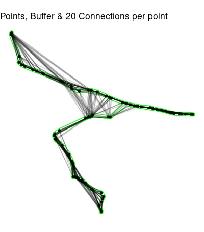
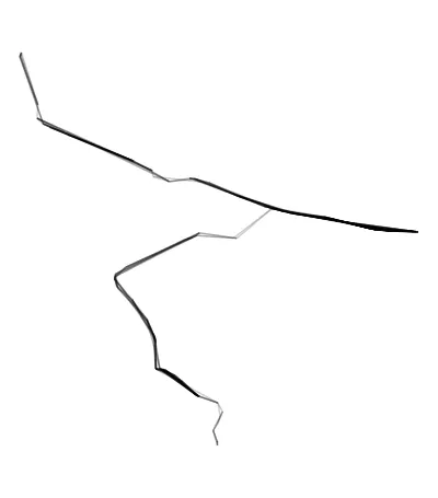
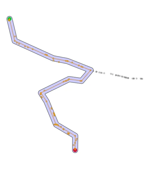
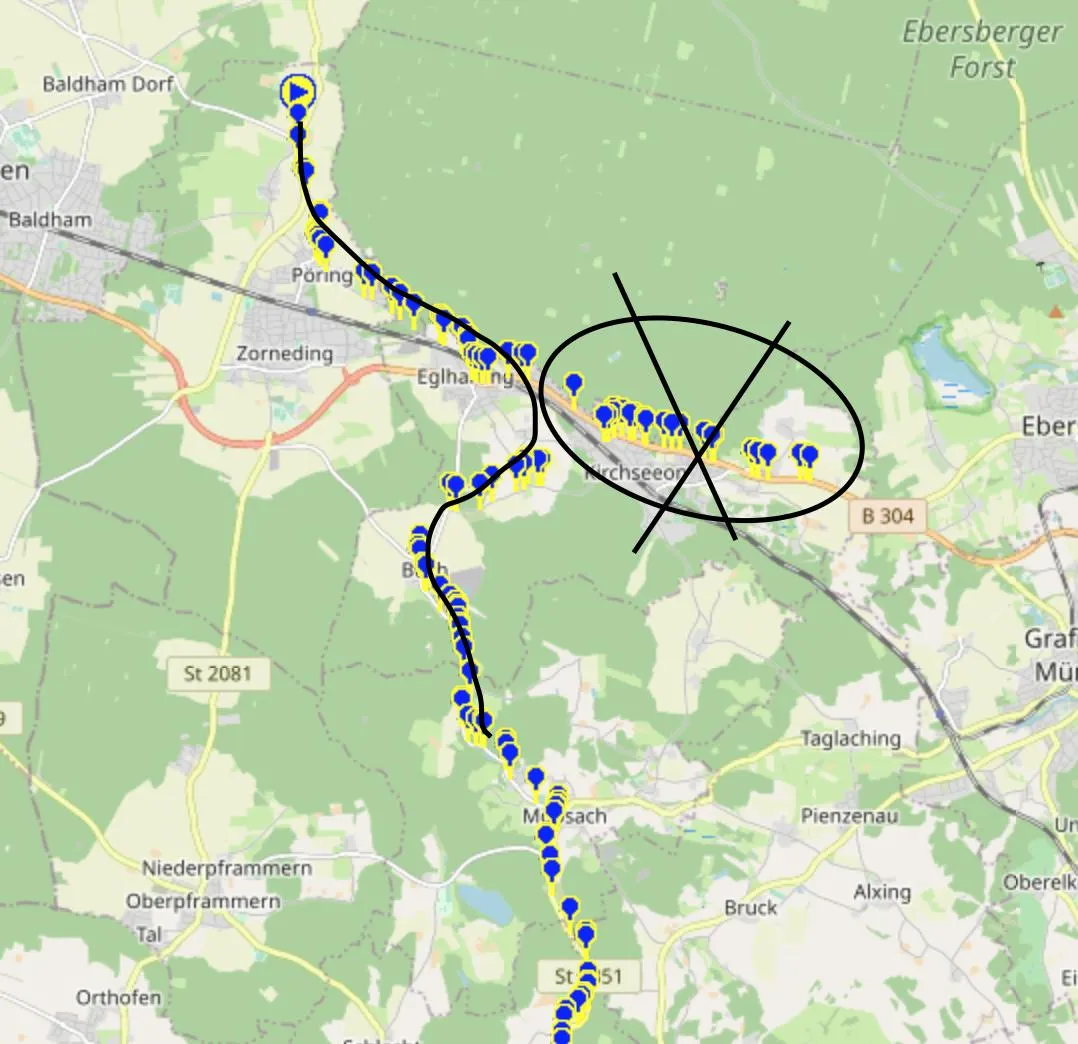
有没有办法过滤掉不属于主路径的部分？如您在图片中所见，我想删除被划掉的部分，同时保留主路径。我已经尝试使用zoo/rolling median，但没有成功。我认为我可以使用某种核来完成这个任务，但我不确定。我还尝试了不同的平滑方法/函数，但这些方法并没有产生期望的结果，反而使情况更糟。 数据中的Dist值可以忽略。

一种方法可能是： 1.取前n个点 2.获取平均/中位数方位角 3.比较n+1点的方位角 4.如果方位角与n个点的平均值相差太大，则舍弃该点。

所以我的路径查找算法的错误是向“前”走然后返回同样的路线。我正在尝试识别和过滤出这种情况。

path<-structure(list(counter = 1:100, lon = c(11.83000844, 11.82986091, 
11.82975536, 11.82968137, 11.82966589, 11.83364579, 11.83346388, 
11.83479848, 11.83630055, 11.84026754, 11.84215965, 11.84530872, 
11.85369492, 11.85449806, 11.85479096, 11.85888555, 11.85908087, 
11.86262424, 11.86715538, 11.86814045, 11.86844252, 11.87138302, 
11.87579809, 11.87736704, 11.87819829, 11.88358436, 11.88923677, 
11.89024638, 11.89091832, 11.90027148, 11.9027736, 11.90408114, 
11.9063466, 11.9068819, 11.90833199, 11.91121547, 11.91204623, 
11.91386018, 11.91657306, 11.91708085, 11.91761264, 11.91204623, 
11.90833199, 11.90739525, 11.90583785, 11.904688, 11.90191917, 
11.90143671, 11.90027148, 11.89806126, 11.89694917, 11.89249712, 
11.88750445, 11.88720159, 11.88532786, 11.87757307, 11.87681905, 
11.86930751, 11.86872102, 11.8676844, 11.86696599, 11.86569006, 
11.85307297, 11.85078596, 11.85065013, 11.85055277, 11.85054529, 
11.85105901, 11.8513188, 11.85441234, 11.85771987, 11.85784653, 
11.85911367, 11.85937322, 11.85957177, 11.85964041, 11.85962915, 
11.8596438, 11.85976783, 11.86056853, 11.86078973, 11.86122148, 
11.86172538, 11.86227576, 11.86392935, 11.86563636, 11.86562302, 
11.86849157, 11.86885719, 11.86901696, 11.86930676, 11.87338922, 
11.87444184, 11.87391755, 11.87329231, 11.8723503, 11.87316759, 
11.87325551, 11.87332646, 11.87329074), lat = c(48.10980039, 
48.10954023, 48.10927434, 48.10891122, 48.10873965, 48.09824039, 
48.09526792, 48.0940306, 48.09328273, 48.09161348, 48.09097173, 
48.08975325, 48.08619985, 48.08594538, 48.08576984, 48.08370241, 
48.08237208, 48.08128785, 48.08204915, 48.08193609, 48.08186387, 
48.08102563, 48.07902278, 48.07827614, 48.07791392, 48.07583181, 
48.07435852, 48.07418376, 48.07408811, 48.07252594, 48.07207418, 
48.07174377, 48.07108668, 48.07094458, 48.07061937, 48.07033965, 
48.07033089, 48.07034706, 48.07025797, 48.07020637, 48.07014061, 
48.07033089, 48.07061937, 48.07081572, 48.07123129, 48.07156883, 
48.07224388, 48.07232886, 48.07252594, 48.07313464, 48.07346191, 
48.07389275, 48.0748072, 48.07488497, 48.07531827, 48.06876325, 
48.06880849, 48.06992189, 48.06935392, 48.0688597, 48.06872843, 
48.0682826, 48.06236784, 48.06083756, 48.06031525, 48.06007589, 
48.05979028, 48.05819348, 48.05773109, 48.05523588, 48.05084893, 
48.0502925, 48.04750087, 48.0471574, 48.04655424, 48.04615637, 
48.04573796, 48.03988503, 48.03985935, 48.03986151, 48.03984645, 
48.0397989, 48.03966795, 48.03925767, 48.03841738, 48.03701502, 
48.03658961, 48.03417456, 48.03394195, 48.03386125, 48.03372952, 
48.03236277, 48.03045774, 48.02935764, 48.02770804, 48.0262546, 
48.02391112, 48.02376389, 48.02361916, 48.02295931), dist = c(16.5491019417617, 
12.387608371535, 13.7541383821868, 33.4916122880205, 6.9703128008864, 
30.9036305788955, 8.61214448946505, 25.0174570393888, 37.1966950033338, 
114.428731827878, 42.6981252797486, 35.484064302826, 46.6949888899517, 
29.3780621124218, 11.3743525290235, 37.7195808156292, 62.6333126726666, 
28.4692721123006, 17.0298455473048, 14.3098664643564, 17.7499631308564, 
87.1393427315571, 60.3089055364667, 41.7849043662927, 87.2691684053224, 
97.1454278187317, 53.9239973250175, 53.8018772046333, 57.751515546603, 
27.3798478555643, 30.6642975040561, 48.4553170757953, 41.9759520786297, 
33.3880134641802, 37.3807049759314, 49.8823206292369, 49.7792541871492, 
61.821997105488, 40.2477260156321, 32.2363477179296, 43.918067054065, 
89.6254564762497, 35.5927710501446, 27.6333379571774, 42.0554883840467, 
45.4018421835631, 4.07647329598549, 52.945234942045, 44.2345694983538, 
63.8855719530995, 37.3036925262838, 11.4985551858961, 47.6500054672646, 
12.488428646998, 13.7372221770588, 24.4479793264376, 71.2384899552303, 
52.9595905197645, 16.8213670893537, 37.0777367654005, 20.1344312201034, 
24.7504557199489, 15.9504355215393, 4.4986704990778, 17.4471004003001, 
9.04823098759565, 25.684547529165, 15.2396067965458, 13.9748972112566, 
88.9846859415509, 15.1658523003296, 18.6262158018174, 8.95876566894735, 
19.8247489326594, 20.4813444727095, 23.6721190072342, 14.4891642200285, 
10.6402985988761, 10.1346051623741, 15.3824252473173, 17.5975390671566, 
15.758052106193, 11.4810033780958, 25.1035007014738, 21.3402595089137, 
28.5373345425722, 11.3907620234039, 7.18155005801645, 13.5078761535753, 
14.0009018934227, 4.09891462242866, 9.47515101787348, 10.755798004242, 
23.9344946865876, 36.4670348302756, 5.53642050027254, 18.2898185695699, 
17.1906059877831, 17.5321948763862, 16.2784860139608)), row.names = c(NA, 
-100L), class = c("data.table", "data.frame"))

更新于2020年9月10日

非常感谢您提出的解决方案。每个解决方案都非常有趣，如果可以的话，我会接受所有的解决方案。

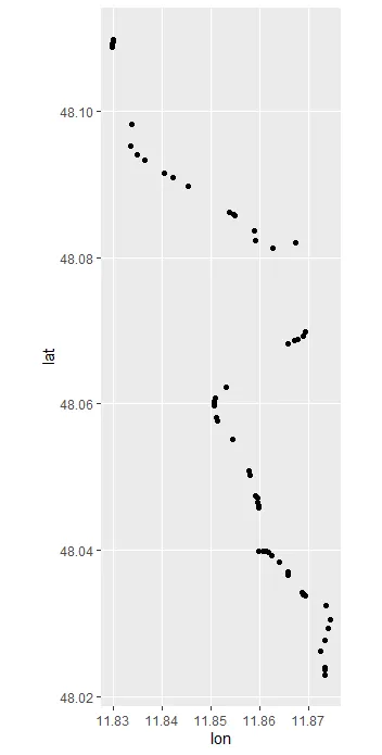
解决方案1由ekoam提供 我真的很喜欢它只依赖于R中的基本包！这是一种有趣的方法，但我必须优化它才能将其应用于整个数据集。我会根据方位角变化划分整个路径，并在过滤器的不同部分上使用此算法并将它们连接在一起。如果我只考虑速度，这将是我选择的方法！

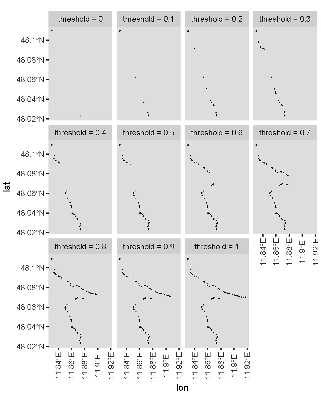
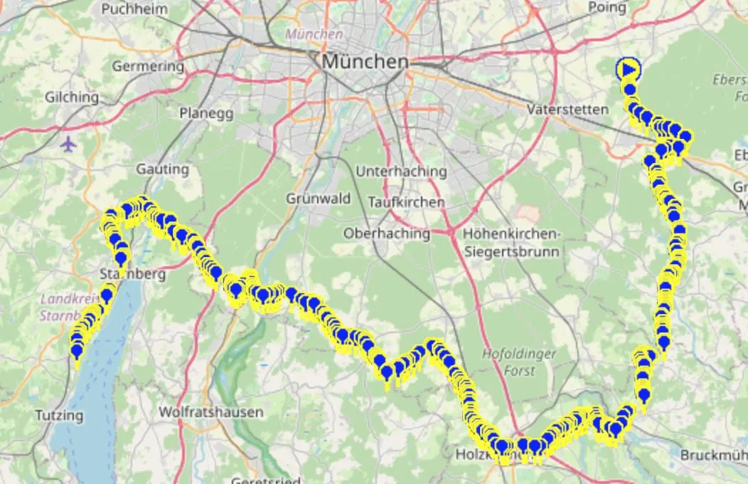
解决方案2由mrhellmann提供 这是一种非常有趣的方法，依赖于非常新鲜的专业软件包。与其他两种相比，它涉及更多的计算，并且产生的结果不如其他两种平滑。我将尝试使用这些软件包，并认为它们有很大的潜力！我调整了K的值，但无法根据绘图删除我想要删除的“尾巴”。

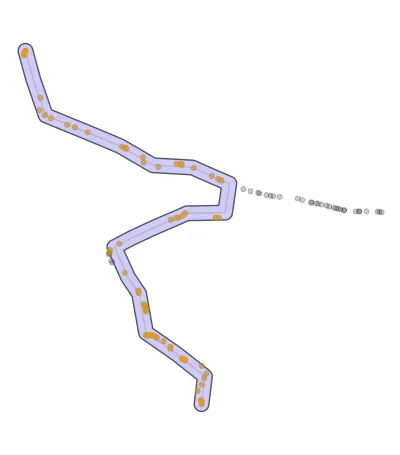
BrianLang的解决方案 Nr3 这个解决方案在整个数据集上立即产生了最好的结果，路径发生了突然变化。它的CPU消耗有点大，但是它可以直接使用而且它效果最好，这就是为什么我会选择这个解决方案作为对这个问题的回答。

非常感谢你们所花费的所有时间来回答这个问题。

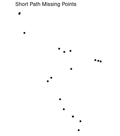
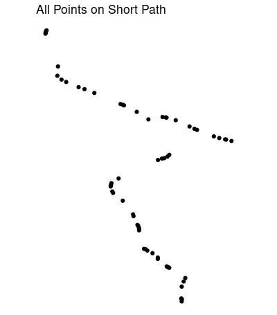
更新 09.10.2020 15:19 实际上，在mrhellmann和BrianLang的提议之间基本上没有区别。 mrhellmann的提议产生了轻微的平滑图形，因为它让其他点存在。 当前的差异是7点。

相比之下，BrianLang的提议

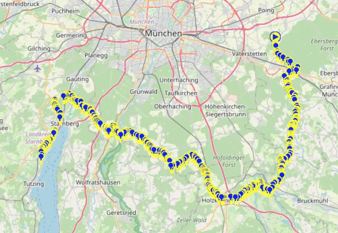
以下是未优化的完整轨迹： mrhellmann提供的解决方案在637个点上运行需要约6秒。BrianLang提供的解决方案也需要6秒运行。 现在唯一的区别在于包的使用和优化的可能性。

- Andreas

---

什么是“主要路径”？在这种情况下，您明显想删除它沿着道路来回走的那一部分，但其他一般情况呢？如果它只是一个小圆环呢？ - pseudospin

你的数据中的“dist”系列是什么？你是否尝试应用一些逻辑/规则来隔离“主路径”之外的点？我们如何知道实际路径不包括那些被X标记圈出来的点——这条路可能会蜿蜒曲折，向东走然后再向西返回来。 - KM_83

也许这会有帮助：https://www.r-spatial.org/r/2019/09/26/spatial-networks.html - Carlos Eduardo Lagosta

我认为@CarlosEduardoLagosta提供的r-spatial链接会有所帮助。如果没有了解你可能要走的路径，这似乎是一项不可能完成的任务，但如果你将你的点映射到道路网络上，你就可以询问起点和终点之间的最短路径，同时尽可能地遵循你提供的航点。 - BrianLang

需要更多关于什么是主路径的定义。多大的转弯半径是可以接受的？只要不是回溯，那就可以吗？如果没有一些定义或更多的例子，就没有答案。 - Roger-123

Answer 1

下面的编辑分别提供了更加正确和完整的答案以及更快的答案。

这个解决方案适用于这种情况，但我不确定它是否适用于形状不同的情况。有一些可以调整的参数可能会找到更好的结果。它严重依赖于sf包和类。

以下代码将：

• 将所有点作为sf对象开始
• 将每个点连接到（可调节的）最近邻居之一
• 删除太远离路径的连接
• 创建一个网络
• 找到最短路径（其中将缺少原始数据中的一些点）
• 获取缺失的点

libary(sf)
library(tidyverse) ## <- heavy, but it's easy to load the whole thing
library(tidygraph) ##  I'm not sure this was needed
library(nngeo)
library(sfnetworks) ## https://github.com/luukvdmeer/sfnetworks


path_sf <- st_as_sf(path, coords = c('lon', 'lat')

# create a buffer around a connected line of our points.
#  used later to filter out unwanted edges of graph
path_buffer <- 
  path_sf %>%
   st_combine() %>%
   st_cast('MULTILINESTRING') %>%
   st_buffer(dist = .001)         ## dist = arg will depend on projection CRS.


# Connect each point to its 20 nearest neighbors,
#  probably overkill, but it works here.  Problems occur when points on the path
#  have very uneven spacing. A workaround would be to st_sample a linestring of the path
connected20 <- st_connect(path_sf, path_sf,
                          ids = st_nn(path_sf, path_sf, k = 20))

到目前为止我们所拥有的：

ggplot() + 
  geom_sf(data = path_sf) + 
  geom_sf(data = path_buffer, color = 'green', alpha = .1) +
  geom_sf(data = connected20, alpha = .1)

现在我们需要消除 path_buffer 以外的连接。

# Remove unwanted edges outside the buffer
edges <- connected20[st_within(connected20,
                               path_buffer,
                               sparse = F),] %>%
  st_as_sf()

ggplot(edges) + geom_sf(alpha = .2) + theme_void()

使用ggplot绘制edges数据，设置透明度为0.2的geom_sf图层，并应用theme_void主题。

## Create a network from the edges
net <- as_sfnetwork(edges, directed = T) ########## directed?

## Use network to find shortest path from the first point to the last. 
## This will exclude some original points,
##  we'll get them back soon.
shortest_path <- st_shortest_paths(net,
                                   path_sf[1,],
                                   path_sf[nrow(path_sf),])

# Probably close to the shortest path, the turn looks long
short_ish <- path_sf[shortest_path$vpath[[1]],] 

< p > short_ish 的情节表明可能缺少一些要点：

# Use this to regain all points on the shortest path
short_buffer <- short_ish %>%
  st_combine() %>%
  st_cast('LINESTRING') %>%
  st_buffer(dist = .001)

short_all <- path_sf[st_within(path_sf, short_buffer, sparse = F), ]

几乎所有可能的最短路径上的点：

调整缓冲距离dist和最近邻居的数量k = 20可能会给您更好的结果。由于某种原因，这会错过分叉口以南的几个点，并且在分叉处可能向东行驶太远。最近邻函数还可以返回距离。删除长于相邻点之间最大距离的连接将有所帮助。 编辑： 在运行上面的代码后，下面的代码应该会得到更好的轨迹。图像包括原始轨迹、最短路径、最短路径上的所有点以及获得这些点的缓冲区。起点为绿色，终点为红色。

## Path buffer as above, dist = .002 instead of .001
path_buffer <- 
  path_sf %>%
  st_combine() %>%
  st_cast('MULTILINESTRING') %>%
  st_buffer(dist = .002)        

### Starting point, 1st point of data
p1 <- net %>% activate('nodes') %>%
  st_as_sf() %>% slice(1)

### Ending point, last point of data
p2 <- net %>% activate('nodes') %>%
  st_as_sf() %>% tail(1)

# New short path
shortest_path2 <- net %>% 
  convert(to_spatial_shortest_paths, p1, p2)
# Buffer again to get all points from original
shortest_path_buffer <- shortest_path2 %>%
  activate(edges) %>% 
  st_as_sf() %>% 
  st_cast('MULTILINESTRING') %>%
  st_combine() %>%
  st_buffer(dist = .0018)

# Shortest path, using all points from original data
all_points_short_path <- path_sf[st_within(path_sf, shortest_path_buffer, sparse = F),]

# Plotting
ggplot() + 
  geom_sf(data = p1, size = 4, color = 'green') + 
  geom_sf(data = p2, size = 4, color = 'red') + 
  geom_sf(data = path_sf, color = 'black', alpha = .2) + 
  geom_sf(data = activate(shortest_path2, 'edges') %>% st_as_sf(), color = 'orange', alhpa = .4) + 
  geom_sf(data = shortest_path_buffer, fill = 'blue', alpha = .2) + 
  geom_sf(data = all_points_short_path, color = 'orange', alpha = .4) +
  theme_void()

编辑2 可能更快，尽管在小数据集上很难确定速度提升了多少。此外，更不可能包含所有正确的点。会漏掉一些原始数据中的点。

path_sf <- st_as_sf(path, coords = c('lon', 'lat'))


# Higher density is slower, but more complete. 
# Higher k will be fooled by winding paths as incorrect edges aren't buffered out
# in the interest of speed.
density = 200
k = 4
  
start <- path_sf[1, ] %>% st_geometry()
end <- path_sf[dim(path_sf)[1],] %>% st_geometry()

path_sf_samp <- path_sf %>%
  st_combine() %>%
  st_cast('LINESTRING') %>%
  st_line_sample(density = density) %>%
  st_cast('POINT') %>%
  st_union(start) %>%
  st_union(end) %>%
  st_cast('POINT')%>%
  st_as_sf()

connected3 <- st_connect(path_sf_samp, path_sf_samp,
                          ids = st_nn(path_sf_samp, path_sf_samp, k = k))

edges <- connected3 %>%
  st_as_sf()

net <- as_sfnetwork(edges, directed = F) ########## directed?

shortest_path <- net %>% 
  convert(to_spatial_shortest_paths, start, end)

shortest_path_buffer <- shortest_path %>%
  activate(edges) %>% 
  st_as_sf() %>% 
  st_cast('MULTILINESTRING') %>%
  st_combine() %>%
  st_buffer(dist = .0018)

all_points_short_path <- path_sf[st_within(path_sf, shortest_path_buffer, sparse = F),]


ggplot() + 
  geom_sf(data = path_sf, color = 'black', alpha = .2) + 
  geom_sf(data = activate(shortest_path, 'edges') %>% st_as_sf(), color = 'orange', alpha = .4) + 
  geom_sf(data = shortest_path_buffer, fill = 'blue', alpha = .2) + 
  geom_sf(data = all_points_short_path, color = 'orange', alpha = .4) +
  theme_void()

- mrhellmann

---

@Andreas 我会在一个小时内编辑帖子并更新，修复问题。 - mrhellmann

发现了我的错误。 - Andreas

@Andreas 编辑2应该更快，尽管不太完整且更容易被曲折的路径所迷惑。根据需要在代码顶部调整density和k。 - mrhellmann

我说，0.519秒更快了。我说你赢了。否则我看不到任何降级。 - Andreas

花了一些时间，但是这是一个有趣的问题。谢谢并祝好运。 - mrhellmann

Answer 2

我将尝试回答这个问题。这里采用的是一个朴素算法。希望其他人能提出比这更好的解决方案。

我猜想，您的GPS轨迹的起点和终点总是在所谓的“主路径”上。如果这个假设是有效的，那么我们可以在这两点之间画一条线并以此作为参考。称这条线为参考线。

算法如下：

1. 对于轨迹的每个点i，计算该点到参考线的距离。将这个距离称为d_i。
2. 制表统计所有d_i的经验分布，并仅选择那些d_i低于该分布的特定分位数的点。将这个分位数称为阈值。使用更高的阈值在逻辑上等同于选择更多的点。
3. 因此，“主路径”是由那些被选择的点定义的路线。

为了计算d_i，我使用来自这个维基百科网页的下列公式：

代码如下：

distan <- function(lon, lat) {
  x1 <- lon[[1L]]; y1 <- lat[[1L]]
  x2 <- tail(lon, 1L); y2 <- tail(lat, 1L)
  dy <- y2 - y1; dx <- x2 - x1
  abs(dy * lon - dx * lat + x2 * y1 - y2 * x1) / sqrt(dy * dy + dx * dx)
}

path_filter <- function(lon, lat, threshold = 0.6) {
  d <- distan(lon, lat)
  th <- quantile(d, threshold, na.rm = TRUE)
  d <= th
}

path_filter 函数返回一个与输入向量长度相同的逻辑向量，你可以像这样使用它（假设 path 是一个 data.table）：

path[path_filter(lon, lat, 0.6), ]

现在让我们看一下不同阈值的主路径结果。我使用以下代码绘制阈值为0、0.1、0.2、...、1的图表。

library(rnaturalearth)
library(ggplot2)
library(dplyr)
library(tidyr)

map <- ne_countries(scale = "small", returnclass = "sf")

df <- 
  path %>% 
  expand(threshold = 0:10 / 10, nesting(counter, lon, lat)) %>% 
  group_by(threshold) %>% 
  filter(path_filter(lon, lat, threshold)) %>% 
  mutate(threshold = paste0("threshold = ", threshold))

ggplot(map) + 
  geom_sf() + 
  geom_point(aes(x = lon, y = lat, group = threshold), size = 0.01, data = df) + 
  coord_sf(xlim = range(df$lon), ylim = range(df$lat)) + 
  facet_wrap(vars(threshold), ncol = 4L) + 
  theme(axis.text.x = element_text(angle = 90, vjust = .5))

这些图形是:

事实上，使用一个更高的阈值会给您更多的点数。对于您的特定情况，我猜您想使用约为0.6的阈值？

- ekoam

---

哇，这太棒了！是的，0.6的阈值看起来不错！我可以接受一点偏离路径。明天我会尝试在整个数据集上使用此解决方案。非常感谢你！看到这个算法如何对方向改变作出反应将是有趣的。 - Andreas

看看这个算法如何对方向变化做出反应会很有趣。我认为我需要根据平均方位角将主路径分成几部分，然后对每一部分应用这个算法。 - Andreas

Answer 3

好的，我已经思考了轴承和轴承之间的差异，并创建了一种方法，它简单地考虑线路(i,i+1)的承载能力和线路(i+1,i+2)的承载能力之间的角度。如果这两个承载能力之间的角度大于某个阈值，则删除点i和i+1。

请看下面的图片：

library(tidyverse)
library(geosphere)

## This function calculates the difference between two bearings
angle_diff <- function(theta1, theta2){
 theta <- abs(theta1 - theta2) %% 360 
 return(ifelse(theta > 180, 360 - theta, theta))
}

## This function removes points (i, i + 1) if the bearing difference 
## between (i, i+1) and (i+1, i+2) is larger than angle 
filter_function <- function(data, angle){
 data %>% ungroup() %>% 
  (function(X)X %>% 
    slice(-(X %>% 
             filter(bearing_diff > angle)  %>%
             select(counter, counter_2) %>%
             unlist()))) 
}


## This function calculates the bearing of the line (i, i+1)
## It also handles the iteration needed in the while-loop
calc_bearing <- function(data, lead_counter = TRUE){
 data %>% 
  mutate(counter = 1:n(),
         lat2 = lead(lat), 
         lon2 = lead(lon),
         counter_2 = lead(counter)) %>%
  rowwise() %>% 
  mutate(bearing = geosphere::bearing(p1 = c(lat, lon),
                                      p2 = c(lat2, lon2))) %>% 
  ungroup() %>%
  mutate(bearing_diff = angle_diff(bearing, lead(bearing)))
}

## this is our max angle
max_angle = 100

## Here is our while loop which cycles though the path,
## removing pairs of points (i, i+1) which have "inconsistent" 
## bearings. 
filtered <- 
 path %>%
 as_tibble() %>% 
 calc_bearing() %>%
 (function(X){
  while(any(X$bearing_diff > max_angle) &
        !is.na(any(X$bearing_diff > max_angle))){
   X <- X %>% 
    filter_function(angle = max_angle) %>%
    calc_bearing()
  }
  X
 })

## Here we plot the new track
ggplot(filtered, aes(lon, lat)) +
 geom_point() +
 coord_map()

- BrianLang

---

我猜测它对偏离起点和终点之间参考线的路径不太敏感。对于某些类型的路径（比如来回跑步），我的方法会返回一个空点列表，这与参考线方法类似。然而，最近邻方法对于来回跑道是可以的。 - BrianLang

你提供的方法是迄今为止最好的，而且它可以直接在我目前尝试的每个路径上运行。@ekoam提供的方法在计算方面是最快的，但我需要将路径分成几部分，并计算这些部分的方位角，然后将此方法应用于路径的各个部分。我认为如果去掉while循环，你的方法可以加速。 - Andreas

或者以某种方式将循环向量化。将其分成几个部分。 - Andreas

最慢的事情肯定是计算方位和方位之间的角度。如果你只在需要计算它们时进行计算，你可以将计算次数从n*k次降至n+k次，其中k表示所需的迭代次数。我认为将其从“while”循环改变会花费比你节省的任何时间都要多得多的时间。切换到data.tables及其实现可能会有所帮助，但我不熟悉如何操作。 - BrianLang

请查看我的eddit以获取结果。 - Andreas

Answer 4

假设您可以在两次访问相同的点之间删除点...

setDT(path)
path[, latlon := paste0(as.character(lat),as.character(lon))]
path[, count := seq(.N), by = latlon]
to_remove  <-  path[latlon %in% path[count == 2, latlon], .(M = max(counter), 
                        m = min(counter)),
                    by = latlon ]
path2 <- path[!counter %in% unique(to_remove[, .(points =  m:M), by = 1:length(to_remove)][, points])]

- MrSmithGoesToWashington

---

我理解你的方法是这样的：你正在寻找被访问两次的相同点？ - Andreas

我在这里看到的问题是：GPS波动在几米之内。因此，两次命中同一点是有点不安全的假设。 - Andreas

我同意你的观点。我不理解的是，在你的问题中，你如何知道你是否可以从一个点到另一个点......我的方法是说明，你不能做之前路径上没有的移动。 - MrSmithGoesToWashington