我正在尝试在R中实现以下卷积,但没有得到预期的结果:
$$
C_{\sigma}[i]=\sum\limits_{k=-P}^P SDL_{\sigma}[i-k,i] \centerdot S[i]
$$
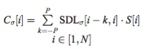
其中$S[i]$是一个频谱强度向量(一个洛伦兹信号/NMR谱),且$i \in [1,N]$,其中$N$是数据点数(例如,实际示例可能有32K个值)。这是Jacob、Deborde和Moing在2013年发表于《分析生物化学》杂志上的第一篇文章的方程式1(DOI 10.1007/s00216-013-6852-y)。
$SDL_{\sigma}$是用于计算洛伦兹曲线的二阶导数的函数,我已按照论文中方程式2的基础进行了实现:
SDL <- function(x, x0, sigma = 0.0005){
    if (!sigma > 0) stop("sigma must be greater than zero.")
    num <- 16 * sigma * ((12 * (x-x0)^2) - sigma^2)
    denom <- pi * ((4 * (x - x0)^2) + sigma^2)^3
    sdl <-  num/denom
    return(sdl)
    }
sigma是半峰宽度,x0是洛伦兹信号的中心。
我相信SDL工作正常(因为返回的值形状类似于经验Savitzky-Golay 2阶导数)。我的问题在于实现$C_{\sigma}$,我已经将其编写为:
CP <- function(S = NULL, X = NULL, method = "SDL", W = 2000, sigma = 0.0005) {
    # S is the spectrum, X is the frequencies, W is the window size (2*P in the eqn above)
    # Compute the requested 2nd derivative
    if (method == "SDL") {

        P <- floor(W/2)
        sdl <- rep(NA_real_, length(X)) # initialize a vector to store the final answer

        for(i in 1:length(X)) {
            # Shrink window if necessary at each extreme
            if ((i + P) > length(X)) P <- (length(X) - i + 1)
            if (i < P) P <- i
            # Assemble the indices corresponding to the window
            idx <- seq(i - P + 1, i + P - 1, 1)
            # Now compute the sdl
            sdl[i] <- sum(SDL(X[idx], X[i], sigma = sigma))
            P <- floor(W/2) # need to reset at the end of each iteration
            }
        }

    if (method == "SG") {
        sdl <- sgolayfilt(S, m = 2)
        }

    # Now convolve!  There is a built-in function for this!
    cp <- convolve(S, sdl, type = "open")
    # The convolution has length 2*(length(S)) - 1 due to zero padding
    # so we need rescale back to the scale of S
    # Not sure if this is the right approach, but it doesn't affect the shape
    cp <- c(cp, 0.0)
    cp <- colMeans(matrix(cp, ncol = length(cp)/2)) # stackoverflow.com/q/32746842/633251
    return(cp)
    }
根据参考文献,为了节省时间,二阶导数的计算仅限于大约2000个数据点的窗口。我认为这部分工作良好,应该只会产生微不足道的扭曲。
下面是整个过程和问题的演示:
require("SpecHelpers")
require("signal")
# Create a Lorentzian curve
loren <- data.frame(x0 = 0, area = 1, gamma = 0.5)
lorentz1 <- makeSpec(loren, plot = FALSE, type = "lorentz", dd = 100, x.range = c(-10, 10))
#
# Compute convolution
x <- lorentz1[1,] # Frequency values
y <- lorentz1[2,] # Intensity values
sig <- 100 * 0.0005 # per the reference
cpSDL <- CP(S = y, X = x, sigma = sig)
sdl <- sgolayfilt(y, m = 2)
cpSG <- CP(S = y, method = "SG")
#
# Plot the original data, compare to convolution product
ylabel <- "data (black), Conv. Prod. SDL (blue), Conv. Prod. SG (red)"
plot(x, y, type = "l", ylab = ylabel, ylim = c(-0.75, 0.75))
lines(x, cpSG*100, col = "red")
lines(x, cpSDL/2e5, col = "blue")
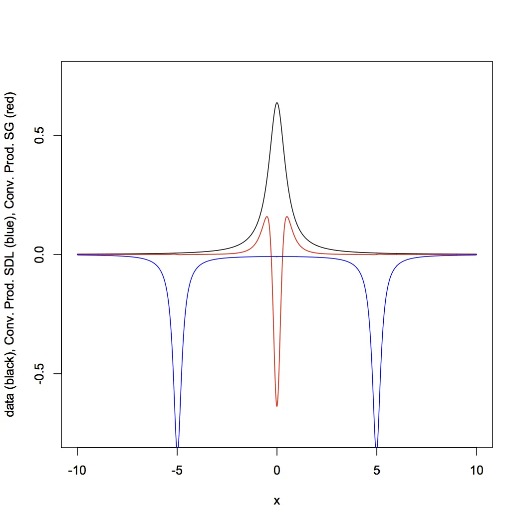
SDL的卷积乘积(蓝色)与使用SG方法的CP的卷积乘积(红色,除了比例不正确外)不相似。我预计使用SDL方法得到的结果应该具有类似的形状但不同的比例。如果您迄今为止一直跟着我,a)感谢您,b)您能看出问题在哪里吗?毫无疑问,我有一个基本的误解。