如何生成一个随机正态分布的整数序列

Question

如何生成一个随机整数，其正态分布围绕着0，类似于np.random.randint()的作用。

np.random.randint(-10, 10)会返回具有离散均匀分布的整数

np.random.normal(0, 0.1, 1)会返回具有正态分布的浮点数

我需要的是两个函数的结合体。

- Ghilas BELHADJ

---

正态分布根据定义是连续的，因此对于这个问题的答案取决于您希望如何将其离散化。一个可能的解决方案是从np.random.normal中进行采样，然后将结果四舍五入为整数。 - Will Vousden

Answer 1

得到一个类似于正态分布的离散分布的另一种方法是从多项式分布中随机抽取样本，其中概率是从正态分布计算出来的。

import scipy.stats as ss
import numpy as np
import matplotlib.pyplot as plt

x = np.arange(-10, 11)
xU, xL = x + 0.5, x - 0.5 
prob = ss.norm.cdf(xU, scale = 3) - ss.norm.cdf(xL, scale = 3)
prob = prob / prob.sum() # normalize the probabilities so their sum is 1
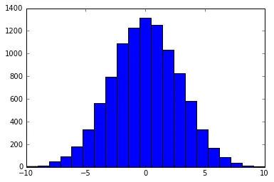
nums = np.random.choice(x, size = 10000, p = prob)
plt.hist(nums, bins = len(x))

在这里，np.random.choice从[-10, 10]中选择一个整数。选择某个元素（比如0）的概率由p(-0.5 < x < 0.5)计算得出，其中x是一个均值为零、标准差为3的正态随机变量。我选择了标准差为3，因为这样p(-10 < x < 10)几乎等于1。

结果看起来像这样：

- ayhan

---

你为什么在 xL 和 xU 中加减 0.5？ - Kenenbek Arzymatov

对于连续分布，P(x=0)=0（对于任何其他数也是如此）。概率定义在区间上。这里，为了将概率与0（和其他整数）相关联，我使用了区间（-0.5，0.5）。这基本上是因为问题要求整数。对于1，它是（0.5，1.5）。 - ayhan

你为什么没有选择 ss.norm.pdf(x, scale=3)？ - Kenenbek Arzymatov

使用这些参数的话，它可以正常工作，但是如果标准偏差变小，你会得到大于1的概率密度函数（PDF），比如说。只要之后进行相同的归一化操作（除以总和），就可以正常使用，但我不想让潜在读者感到困惑，因为PDF实际上并不表示概率（这就是它可能大于1的原因），所以我想使用实际的概率值。 - ayhan

Answer 2

可能可以通过生成一个四舍五入到整数的截断正态分布来得到类似的分布。以下是使用scipy的truncnorm()的示例。

import numpy as np
from scipy.stats import truncnorm
import matplotlib.pyplot as plt

scale = 3.
range = 10
size = 100000

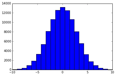
X = truncnorm(a=-range/scale, b=+range/scale, scale=scale).rvs(size=size)
X = X.round().astype(int)

让我们看看它的样子

bins = 2 * range + 1
plt.hist(X, bins)

- bakkal

---

我感谢@ayhan和bakkal的回复。请注意，我只是为了增加我的知识而提出这个问题，我并不想冒犯任何一个答案。从图表上看，Bakkal的更对称。它们两个似乎都足够好，并且从代码上看同样有效。但是我的理解比较薄弱。是否有客观上更好的方法？ - Robert Lugg

@RobertLugg 相对较高的对称性可能是由于样本大小较大。话虽如此，我认为这个答案中的代码更简单。 - bakkal

请注意，此代码将覆盖Python的range函数。尽量使用中性的变量名称。 - Rriskit

虽然代码更简单，但运行速度也比较慢。在我的测试中，它比Ayhan的解决方案慢了大约100倍。不过，生成10,000个数字50次仍需要3秒钟的时间。因此，在许多情况下这是可以接受的。 - Pablo

这个答案有点错误，因为第一个和最后一个桶的概率会比其他桶低。这是因为 X.round() 会使用 0.5 作为截止点进行自然舍入，而所有生成的实数值都在 [a,b) 范围内。要解决这个问题，请改用 np.floor(X).astype(int)，它将产生 [a,b) 范围内等概率的整数值。 - bricklore

Answer 3

这里的被接受的答案是可行的，但我也尝试了Will Vousden的解决方案，它也运行良好：

import numpy as np

# Generate Distribution:
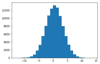
randomNums = np.random.normal(scale=3, size=100000)
randomInts = np.round(randomNums)

# Plot:
axis = np.arange(start=min(randomInts), stop = max(randomInts) + 1)
plt.hist(randomInts, bins = axis)

- stephan

---

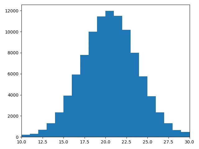
与其生成“随机数”并将它们四舍五入为“整数”（实际上是以.0结尾的实数），不如使用randomInts = np.random.normal(loc=10, scale=3, size=10000).astype(int)-10来生成真正的整数。注意，然而，必须使用非0的loc值来生成值（并通过减去loc将其返回到0），否则您将得到太多恰好等于0的结果。 - Dave Land

Answer 4

旧问题新答案：

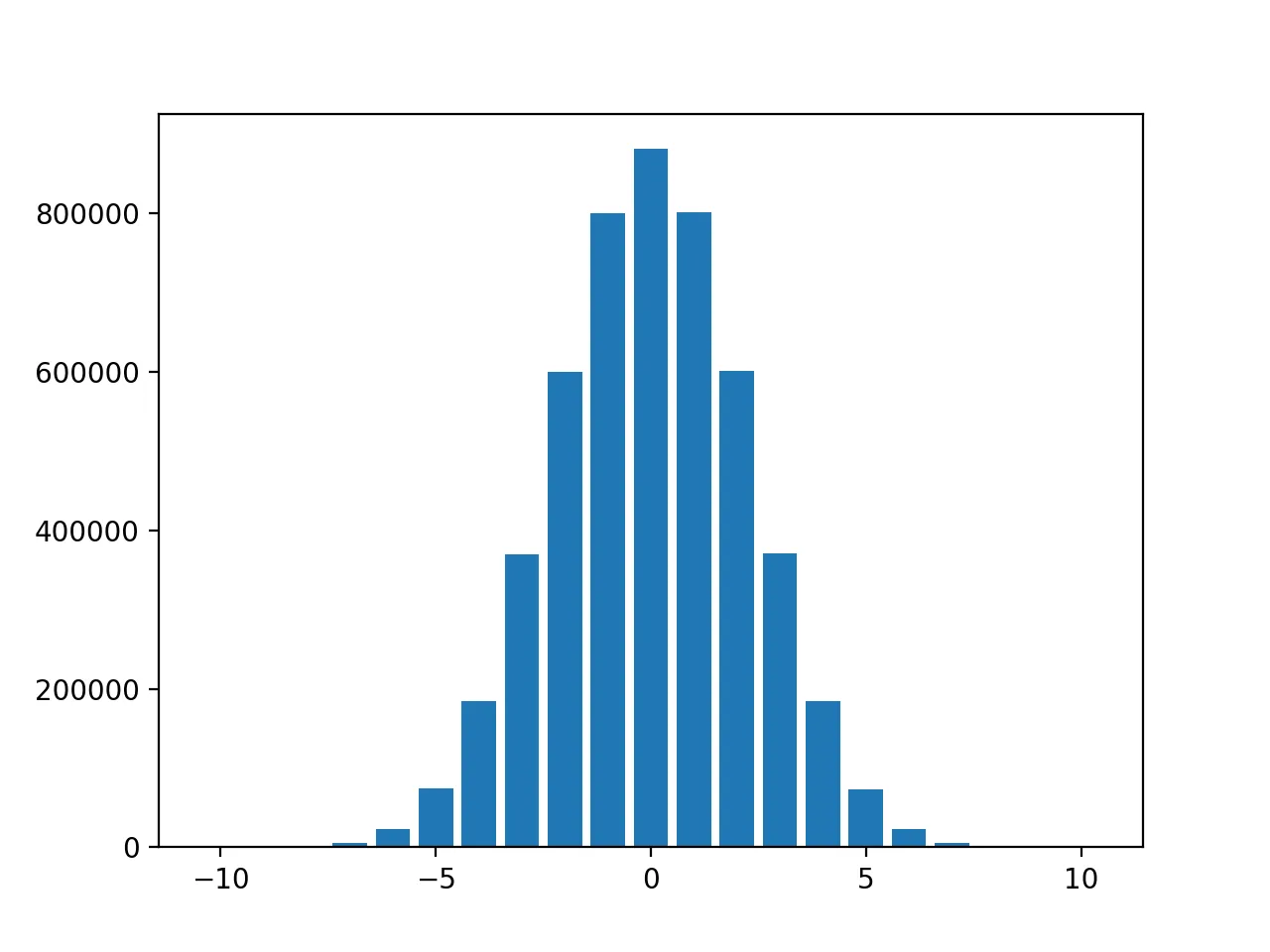
对于整数集合{-10，-9，...，9，10}的钟形分布，您可以使用n = 20和p = 0.5的二项分布，并从样本中减去10。

例如，

In [167]: import numpy as np

In [168]: import matplotlib.pyplot as plt

In [169]: rng = np.random.default_rng()

In [170]: N = 5000000   # Number of samples to generate

In [171]: samples = rng.binomial(n=20, p=0.5, size=N) - 10

In [172]: samples.min(), samples.max()
Out[172]: (-10, 10)

请注意，-10或10的概率非常低，因此您不一定会在任何给定样本中看到它们，特别是如果您使用较小的N。

np.bincount()是生成一组小的非负整数的直方图的有效方法：

In [173]: counts = np.bincount(samples + 10, minlength=20)

In [174]: counts
Out[174]: 
array([     4,    104,    889,   5517,  22861,  73805, 184473, 369441,
       599945, 800265, 881140, 801904, 600813, 370368, 185082,  73635,
        23325,   5399,    931,     95,      4])

In [175]: plt.bar(np.arange(-10, 11), counts)
Out[175]: <BarContainer object of 21 artists>

- Warren Weckesser

---

我找不到已导入的 rng，但它应该是这个：rng = np.random.default_rng()，这可能代表“默认随机数生成器”。https://devdocs.io/numpy~1.20/reference/random/index#random-quick-start - Stefan_EOX

感谢您指出这一点，@Stefan_EOX。我已更新代码以包括rng的创建。 - Warren Weckesser

Answer 5

我不确定在scipy生成器中是否有选择var-type的选项可以生成，但通常的生成可以使用scipy.stats。

# Generate pseudodata  from a single normal distribution
import scipy
from scipy import stats
import numpy as np
import matplotlib.pyplot as plt

dist_mean = 0.0
dist_std = 0.5
n_events = 500

toy_data = scipy.stats.norm.rvs(dist_mean, dist_std, size=n_events)
toy_data2 = [[i, j] for i, j in enumerate(toy_data )]

arr = np.array(toy_data2)
print("sample:\n", arr[1:500, 0])
print("bin:\n",arr[1:500, 1])
plt.scatter(arr[1:501, 1], arr[1:501, 0])
plt.xlabel("bin")
plt.ylabel("sample")
plt.show()

或者以这种方式（也没有dtype选择的选项）：

import matplotlib.pyplot as plt

mu, sigma = 0, 0.1 # mean and standard deviation
s = np.random.normal(mu, sigma, 500)

count, bins, ignored = plt.hist(s, 30, density=True)
plt.show()
print(bins)     # <<<<<<<<<<

plt.plot(bins, 1/(sigma * np.sqrt(2 * np.pi)) * np.exp( - (bins - mu)**2 / (2 * sigma**2) ),
          linewidth=2, color='r')
plt.show()

没有可视化的情况下，最常见的方式是（也没有指出变量类型的可能性）

bins = np.random.normal(3, 2.5, size=(10, 1))

可以编写一个包装类来使用给定的变量数据类型实例化容器（例如，通过将浮点数四舍五入为整数，如上所述）...

- JeeyCi

Answer 6

这个版本在数学上不正确（因为你切掉了钟形曲线），但如果不需要那么精确，它可以快速而容易地完成工作并且易于理解：

def draw_random_normal_int(low:int, high:int):

    # generate a random normal number (float)
    normal = np.random.normal(loc=0, scale=1, size=1)

    # clip to -3, 3 (where the bell with mean 0 and std 1 is very close to zero
    normal = -3 if normal < -3 else normal
    normal = 3 if normal > 3 else normal

    # scale range of 6 (-3..3) to range of low-high
    scaling_factor = (high-low) / 6
    normal_scaled = normal * scaling_factor

    # center around mean of range of low high
    normal_scaled += low + (high-low)/2

    # then round and return
    return np.round(normal_scaled)

绘制10万个数字的结果如下直方图：

- Maikefer

Answer 7

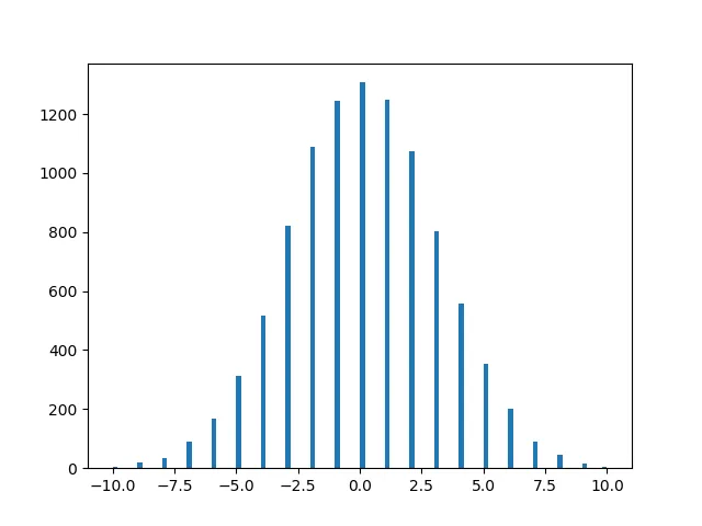
在这里，我们从钟形曲线中获取值。

代码：

#--------*---------*---------*---------*---------*---------*---------*---------*
# Desc: Discretize a normal distribution centered at 0
#--------*---------*---------*---------*---------*---------*---------*---------*

import sys
import random
from math import sqrt, pi
import numpy as np
import matplotlib.pyplot as plt

def gaussian(x, var):
    k1 = np.power(x, 2)
    k2 = -k1/(2*var)
    return (1./(sqrt(2. * pi * var))) * np.exp(k2)

#--------*---------*---------*---------*---------*---------*---------*---------#
while 1:#                          M A I N L I N E                             #
#--------*---------*---------*---------*---------*---------*---------*---------#
#                                  # probability density function
#                                  #   for discrete normal RV
    pdf_DGV = []
    pdf_DGW = []    
    var = 9
    tot = 0    
#                                  # create 'rough' gaussian
    for i in range(-var - 1, var + 2):
        if i ==  -var - 1:
            r_pdf = + gaussian(i, 9) + gaussian(i - 1, 9) + gaussian(i - 2, 9)
        elif i == var + 1:
            r_pdf = + gaussian(i, 9) + gaussian(i + 1, 9) + gaussian(i + 2, 9)
        else:
            r_pdf = gaussian(i, 9)
        tot = tot + r_pdf
        pdf_DGV.append(i)
        pdf_DGW.append(r_pdf)
        print(i, r_pdf)
#                                  # amusing how close tot is to 1!
    print('\nRough total = ', tot)
#                                  # no need to normalize with Python 3.6,
#                                  #   but can't help ourselves
    for i in range(0,len(pdf_DGW)):
        pdf_DGW[i] = pdf_DGW[i]/tot
#                                  # print out pdf weights
#                                  #   for out discrte gaussian
    print('\npdf:\n')
    print(pdf_DGW)

#                                  # plot random variable action
    rv_samples = random.choices(pdf_DGV, pdf_DGW, k=10000)
    plt.hist(rv_samples, bins = 100)
    plt.show()
    sys.exit()

输出：

-10 0.0007187932912256041
-9 0.001477282803979336
-8 0.003798662007932481
-7 0.008740629697903166
-6 0.017996988837729353
-5 0.03315904626424957
-4 0.05467002489199788
-3 0.0806569081730478
-2 0.10648266850745075
-1 0.12579440923099774
0 0.1329807601338109
1 0.12579440923099774
2 0.10648266850745075
3 0.0806569081730478
4 0.05467002489199788
5 0.03315904626424957
6 0.017996988837729353
7 0.008740629697903166
8 0.003798662007932481
9 0.001477282803979336
10 0.0007187932912256041

Rough total =  0.9999715875468381

pdf:

[0.000718813714486599, 0.0014773247784004072, 0.003798769940305483, 0.008740878047691289, 0.017997500190860556, 0.033159988420867426, 0.05467157824565407, 0.08065919989878699, 0.10648569402724471, 0.12579798346031068, 0.13298453855078374, 0.12579798346031068, 0.10648569402724471, 0.08065919989878699, 0.05467157824565407, 0.033159988420867426, 0.017997500190860556, 0.008740878047691289, 0.003798769940305483, 0.0014773247784004072, 0.000718813714486599]

- CopyPasteIt