我想为iPhone开发一个吉他调音器应用程序。我的目标是找到吉他弦所产生的声音的基频。我使用了苹果提供的aurioTouch示例代码的一些部分来计算频谱,并找到具有最高幅度的频率。对于纯声音(仅有一个频率的声音),它运行良好,但对于吉他弦的声音,它会产生错误的结果。我已经了解到这是由于吉他弦产生的泛音可能具有比基频更高的振幅。如何找到基频以使其适用于吉他弦?是否有C / C ++ / Obj-C的开源库可用于音频分析(或信号处理)?
如何找到吉他弦音的基频?
17
- Mircea
5
1我不是音乐家,但如果你想做一个调音器,为什么需要识别和弦?一次调一个字符串不是更容易吗? - mtrw
@mtrw 这是拼写错误... 应该是 "cord" 而不是 "chord"... 对于误解我感到抱歉。 - Mircea
7请修改错误并使用术语“字符串”以避免进一步的混淆。 - Clifford
这个问题和答案非常有帮助。它的回答方式已经(几乎)与Objective-C无关了。如果您能删除Objective-C标签,并从问题中删除Objective-C,以便更广泛的受众更容易找到,那就太好了。 - AudioDroid
如果你找到了 iPhone 的解决方案,请帮我一下。 - tryKuldeepTanwar
3个回答
47
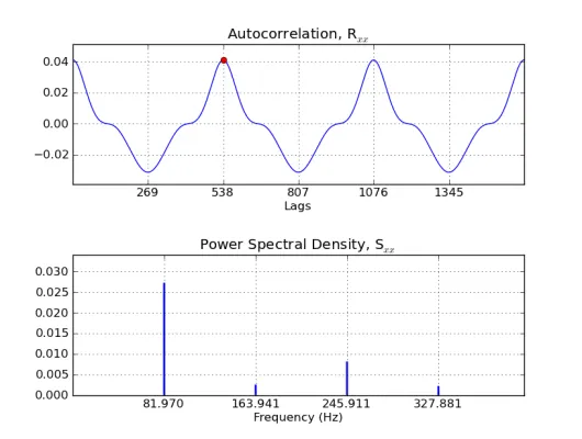
您可以使用信号的自相关函数,它是DFT幅度平方的反变换。如果您以44100个样本/秒的速率采样,则82.4 Hz的基频约为535个样本,而1479.98 Hz约为30个样本。在该范围内(例如28到560),寻找最高峰正向滞后。确保您的窗口至少为最长基频的两个周期,这里是1070个样本。将其取到下一个二的幂,即2048个样本的缓冲区。为了获得更好的频率分辨率和不那么有偏差的估计,使用更长的缓冲区,但不要太长,以至于信号不再近似稳态。以下是Python的示例:
from pylab import *
import wave

fs = 44100.0   # sample rate
K = 3          # number of windows
L = 8192       # 1st pass window overlap, 50%
M = 16384      # 1st pass window length
N = 32768      # 1st pass DFT lenth: acyclic correlation

# load a sample of guitar playing an open string 6
# with a fundamental frequency of 82.4 Hz (in theory),
# but this sample is actually at about 81.97 Hz
g = fromstring(wave.open('dist_gtr_6.wav').readframes(-1),
               dtype='int16')
g = g / float64(max(abs(g)))    # normalize to +/- 1.0
mi = len(g) / 4                 # start index

def welch(x, w, L, N):
    # Welch's method
    M = len(w)
    K = (len(x) - L) / (M - L)
    Xsq = zeros(N/2+1)                  # len(N-point rfft) = N/2+1
    for k in range(K):
        m = k * ( M - L)
        xt = w * x[m:m+M]
        # use rfft for efficiency (assumes x is real-valued)
        Xsq = Xsq + abs(rfft(xt, N)) ** 2
    Xsq = Xsq / K
    Wsq = abs(rfft(w, N)) ** 2
    bias = irfft(Wsq)                   # for unbiasing Rxx and Sxx
    p = dot(x,x) / len(x)               # avg power, used as a check
    return Xsq, bias, p

# first pass: acyclic autocorrelation
x = g[mi:mi + K*M - (K-1)*L]        # len(x) = 32768
w = hamming(M)                      # hamming[m] = 0.54 - 0.46*cos(2*pi*m/M)
                                    # reduces the side lobes in DFT
Xsq, bias, p = welch(x, w, L, N)
Rxx = irfft(Xsq)                    # acyclic autocorrelation
Rxx = Rxx / bias                    # unbias (bias is tapered)
mp = argmax(Rxx[28:561]) + 28       # index of 1st peak in 28 to 560

# 2nd pass: cyclic autocorrelation
N = M = L - (L % mp)                # window an integer number of periods
                                    # shortened to ~8192 for stationarity
x = g[mi:mi+K*M]                    # data for K windows
w = ones(M); L = 0                  # rectangular, non-overlaping
Xsq, bias, p = welch(x, w, L, N)
Rxx = irfft(Xsq)                    # cyclic autocorrelation
Rxx = Rxx / bias                    # unbias (bias is constant)
mp = argmax(Rxx[28:561]) + 28       # index of 1st peak in 28 to 560

Sxx = Xsq / bias[0]
Sxx[1:-1] = 2 * Sxx[1:-1]           # fold the freq axis
Sxx = Sxx / N                       # normalize S for avg power
n0 = N / mp
np = argmax(Sxx[n0-2:n0+3]) + n0-2  # bin of the nearest peak power

# check
print "\nAverage Power"
print "  p:", p
print "Rxx:", Rxx[0]                # should equal dot product, p
print "Sxx:", sum(Sxx), '\n'        # should equal Rxx[0]

figure().subplots_adjust(hspace=0.5)
subplot2grid((2,1), (0,0))
title('Autocorrelation, R$_{xx}$'); xlabel('Lags')
mr = r_[:3 * mp]
plot(Rxx[mr]); plot(mp, Rxx[mp], 'ro')
xticks(mp/2 * r_[1:6])
grid(); axis('tight'); ylim(1.25*min(Rxx), 1.25*max(Rxx))

subplot2grid((2,1), (1,0))
title('Power Spectral Density, S$_{xx}$'); xlabel('Frequency (Hz)')
fr = r_[:5 * np]; f = fs * fr / N;
vlines(f, 0, Sxx[fr], colors='b', linewidth=2)
xticks((fs * np/N  * r_[1:5]).round(3))
grid(); axis('tight'); ylim(0,1.25*max(Sxx[fr]))
show()
Average Power
  p: 0.0410611012542
Rxx: 0.0410611012542
Sxx: 0.0410611012542
编辑:更新为使用Welch方法估计自相关。重叠窗口补偿汉明窗口。还计算了汉明窗口的锥形偏差以对自相关进行无偏置化。
编辑:添加了第二次通过循环相关清除功率谱密度。该过程使用3个不重叠的矩形窗口长度为538*15 = 8070(足够短,几乎静止)。循环相关的偏差是一个常数,而不是汉明窗口的锥形偏差。
- Eryk Sun
2
1当基频小于谐波(或完全缺失)时,这种技术是否有效? - mtrw
1如果您有一个2 Hz的泛音和一个3 Hz的泛音,三角形外观的结果波形仍然会每1秒重复一次,即使没有任何1 Hz正弦内容,长时间窗口的自相关也能找到。 - hotpaw2
4
在和弦中查找音高比估算一次弦或一个音符的音高要困难得多。和弦中多个音符的泛音可能会相互重叠和交错。常见和弦中的所有音符本身都可能是一个或多个不存在低音调的泛音频率。
对于单个音符,自相关是一些吉他调音器使用的常见技术。但是,在自相关中,您必须意识到一些潜在的八度不确定性,因为吉他可能会产生不谐波和衰减的泛音,因此从一个音高周期到另一个音高周期无法完全匹配。cepstrum和Harmonic Product Spectrum是另外两种音高估计方法,它们可能具有不同的问题,这取决于吉他和音符。 RAPT似乎是一种更健壮的音高估计算法。YIN是另一种。
另外,Objective C是ANSI C的超集。因此,您可以在Objective C应用程序中使用任何您发现的C DSP例程进行音高估计。
对于单个音符,自相关是一些吉他调音器使用的常见技术。但是,在自相关中,您必须意识到一些潜在的八度不确定性,因为吉他可能会产生不谐波和衰减的泛音,因此从一个音高周期到另一个音高周期无法完全匹配。cepstrum和Harmonic Product Spectrum是另外两种音高估计方法,它们可能具有不同的问题,这取决于吉他和音符。 RAPT似乎是一种更健壮的音高估计算法。YIN是另一种。
另外,Objective C是ANSI C的超集。因此,您可以在Objective C应用程序中使用任何您发现的C DSP例程进行音高估计。
- hotpaw2
2
@eryksun 你是对的... 我本意是用 "cord" 作为 "string" 的同义词。 - Mircea
谢谢你的回答,我很抱歉出现了“chord”和“cord”的错误。 - Mircea
网页内容由stack overflow 提供, 点击上面的可以查看英文原文,
原文链接
原文链接