在多边形内描绘不规则数据轮廓

Question

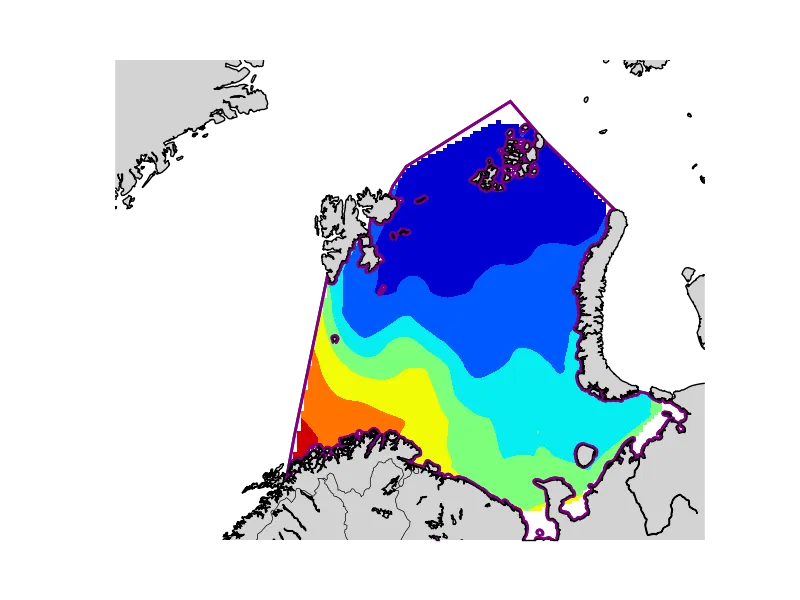
我需要在多边形内创建海表温度（SST）数据的填充等高线图，但是我不确定最佳方法。我有三个包含X、Y和SST数据的1D数组，我使用以下代码创建附图：

p=PatchCollection(mypatches,color='none', alpha=1.0,edgecolor="purple",linewidth=2.0)
levels=np.arange(SST.min(),SST.max(),0.2)
datamap=mymap.scatter(x,y,c=SST, s=55, vmin=-2,vmax=3,alpha=1.0)

我希望能够将这些数据绘制成填充轮廓图(contourf而不是散点)，并将其限制(剪切)在多边形边界内(紫色线)。非常感谢您提供如何实现此目标的建议。

更新： 我最初尝试使用griddata，但无法使其正常工作。然而，基于@eatHam提供的答案，我决定再试一次。当我选择方法'cubic'时，我的scipy griddata无法正常工作，因为它在网格化时一直挂起，但当我切换到matplotlib.mlab.griddata并使用'linear'插值时，它就可以工作了。关于遮罩边界的建议提供了一个非常粗略且不够准确的解决方案，不如我所期望的那样。 我搜索了有关如何剪切matplotlib中轮廓的选项，并在@pelson的答案中找到了一个答案，该答案在此链接中提供。我尝试了隐含在“轮廓集本身没有set_clip_path方法，但是您可以遍历每个轮廓集并设置它们各自的剪切路径”的建议解决方案。我的新的最终解决方案如下所示(请参见下图)：

  p=PatchCollection(mypatches,color='none', alpha=1.0,edgecolor="purple",linewidth=2.0)
  levels=np.arange(SST.min(),SST.max(),0.2)
  grid_x, grid_y = np.mgrid[x.min()-0.5*(x.min()):x.max()+0.5*(x.max()):200j,
                          y.min()-0.5*(y.min()):y.max()+0.5*(y.max()):200j]
  grid_z = griddata(x,y,SST,grid_x,grid_y)

  cs=mymap.contourf(grid_x, grid_y, grid_z)

  for poly in mypatches:
      for artist in ax.get_children():
          artist.set_clip_path(poly)

      ax.add_patch(poly)
  mymap.drawcountries()
  mymap.drawcoastlines()
  mymap.fillcontinents(color='lightgrey',lake_color='none')
  mymap.drawmapboundary(fill_color='none')

这个解决方案可以在北部边缘部分进行改进，以推断极端边缘。欢迎提出如何真正“填补”整个多边形的建议。我也想知道为什么mlab有效而scipy无效。

- Trond Kristiansen

---

你尝试过哪些插值方法？ - tacaswell

griddata 的 scipy 和 mlab 版本及不同方法，这一点并不令人惊讶。我认为在数据范围之外进行插值的问题更多地涉及基本问题，并且需要采用可疑的方法来解决；) - tacaswell

Answer 1

我会使用 scipy.griddata 对数据进行插值。你可以将区域（mypatches）外的部分设置为np.nan。然后只需使用pyplot.contour进行绘制即可。

import numpy as np
import matplotlib.pyplot as plt
from scipy.interpolate import griddata

def sst_data(x, y):
    return x*(1-x)*np.cos(4*np.pi*x) * np.sin(4*np.pi*y**2)**2

                         #replace with ...
x = np.random.rand(1000) #... your x
y = np.random.rand(1000) #... your y
sst = sst_data(x, y)     #... your sst

# interpolate to a grid
grid_x, grid_y = np.mgrid[0:1:100j, 0:1:200j] 
grid_z = griddata((x,y), sst, (grid_x, grid_y), method='cubic')

# mask out the area outside of your region
nr, nc = grid_z.shape
grid_z[-nr//3:, -nc//3:] = np.nan

plt.contourf(grid_x, grid_y, grid_z)

plt.show()

编辑：在plt.contourf()调用中更改了变量名称（之前是..（grid_z，grid_y，grid_z））

- thorink

---

你的建议让我找到了正确的方向，所以我接受了你的答案。 - Trond Kristiansen