双重嵌套在tidyverse中

Question

使用Wickham在《R数据科学中的purrr介绍》中的示例，我正在尝试创建一个双重嵌套列表。

library(gapminder)
library(purrr)
library(tidyr)
gapminder
nest_data <- gapminder %>% group_by(continent) %>% nest(.key = by_continent) 

我该如何进一步嵌套国家，使nest_data包含按大陆分类的数据和一个新的按国家分类的层次，最终包括按年份分类的表格？

此外，在创建了这个gapminder数据结构之后，您将如何为每个国家运行书中的回归模型示例？（参见本章）

- Misha

---

你为什么不能在按照大陆和国家分组之后直接嵌套呢？这似乎更容易处理。如果你真的想要嵌套列表列，那么可以尝试使用 nest_data %>% mutate(by_continent = map(by_continent, ~.x %>% group_by(country) %>% nest(.key = by_country)))。 - aosmith

感谢您的帮助。结构只是试图理解列表列的问题。您的命令非常有效。但是，我不确定我是否理解了为什么。我尝试了类似的东西，但只是用 ~ 而不是 ~.x 。x 是什么意思？此外，如果我现在想要对每个国家运行回归而不使用 unnesting 并将结果放在 by_country 中，该怎么做？ - Misha

我曾经看到在 map 中既有使用 . 又有使用 .x 的情况，但我通常使用 .x，因为这是文档中的写法。也许是由于 mutate 包装器导致了混淆，所以出现了使用 . 的情况。至于从嵌套表格中按国家获取模型的问题，很快就会变得混乱。我运行了以下代码：mutate(nested_again, models = map(by_continent, "by_country") %>% at_depth(2, ~lm(lifeExp ~ year, data = .x)))。 - aosmith

Answer 1

以下是我的解决方案及相关说明。

library(gapminder)
library(purrr)
library(tidyr)
library(broom)

nest_data <- gapminder %>% group_by(continent) %>% nest(.key = by_continent) 

第一个问题是：如何将by_country嵌套在by_continent内

@aosmith在评论中提供了很好的解决方案

nested_again<-
nest_data %>% mutate(by_continent = map(by_continent, ~.x %>% 
                                          group_by(country) %>% 
                                          nest(.key = by_country)))
# Level 1
nested_again
# # A tibble: 5 × 2
# continent      by_continent
# <fctr>            <list>
#   1      Asia <tibble [33 × 2]>
#   2    Europe <tibble [30 × 2]>
#   3    Africa <tibble [52 × 2]>
#   4  Americas <tibble [25 × 2]>
#   5   Oceania  <tibble [2 × 2]>

# Level 2
nested_again %>% unnest %>% slice(1:2)
# # A tibble: 2 × 3
# continent     country        by_country
# <fctr>      <fctr>            <list>
#   1      Asia Afghanistan <tibble [12 × 4]>
#   2      Asia     Bahrain <tibble [12 × 4]>

第二个问题：如何在更深层次上应用回归模型（并保存在tibble中，我猜）

@aosmith提供的解决方案（我称之为sol1）：

sol1<-mutate(nested_again, models = map(by_continent, "by_country") %>%
         at_depth(2, ~lm(lifeExp ~ year, data = .x)))

sol1
# # A tibble: 5 × 3
# continent      by_continent      models
# <fctr>            <list>      <list>
#   1      Asia <tibble [33 × 2]> <list [33]>
#   2    Europe <tibble [30 × 2]> <list [30]>
#   3    Africa <tibble [52 × 2]> <list [52]>
#   4  Americas <tibble [25 × 2]> <list [25]>
#   5   Oceania  <tibble [2 × 2]>  <list [2]>

sol1 %>% unnest(models)
# Error: Each column must either be a list of vectors or a list of data frames [models]
sol1 %>% unnest(by_continent) %>% slice(1:2)
# # A tibble: 2 × 3
#   continent     country        by_country
#      <fctr>      <fctr>            <list>
# 1      Asia Afghanistan <tibble [12 × 4]>
# 2      Asia     Bahrain <tibble [12 × 4]>

这个解决方案正在按照预期执行，但是由于该信息嵌套在第二级别中，没有简单的过滤国家的方法。

我建议采用第2种解决方案，基于@aomith对第一个问题的解决方案。

sol2<-nested_again %>% mutate(by_continent = map(by_continent, ~.x %>% 
                  mutate(models = map(by_country, ~lm(lifeExp ~ year, data = .x) )) ))
sol2
# # A tibble: 5 × 2
#   continent      by_continent
#      <fctr>            <list>
# 1      Asia <tibble [33 × 4]>
# 2    Europe <tibble [30 × 4]>
# 3    Africa <tibble [52 × 4]>
# 4  Americas <tibble [25 × 4]>
# 5   Oceania  <tibble [2 × 4]>

sol2 %>% unnest %>% slice(1:2)
# # A tibble: 2 × 4
#   continent     country        by_country   models
#      <fctr>      <fctr>            <list>   <list>
# 1      Asia Afghanistan <tibble [12 × 4]> <S3: lm>
# 2      Asia     Bahrain <tibble [12 × 4]> <S3: lm>

sol2 %>% unnest %>% unnest(by_country) %>% colnames
# [1] "continent" "country"   "year"      "lifeExp"   "pop"      
# [6] "gdpPercap"

# get model by specific country
sol2 %>% unnest %>% filter(country == "Brazil") %$% models %>% extract2(1)
# Call:
#   lm(formula = lifeExp ~ year, data = .x)
# 
# Coefficients:
#   (Intercept)         year  
# -709.9427       0.3901

# summary with broom::tidy
sol2 %>% unnest %>% filter(country == "Brazil") %$% models %>%
  extract2(1) %>% tidy
#          term     estimate    std.error statistic      p.value
# 1 (Intercept) -709.9426860 10.801042821 -65.72909 1.617791e-14
# 2        year    0.3900895  0.005456243  71.49417 6.990433e-15

我们可以整理所有的模型并保存在数据中以便于绘图或筛选。

sol2 %<>% mutate(by_continent = map(by_continent, ~.x %>% 
        mutate(tidymodels = map(models, tidy )) ))

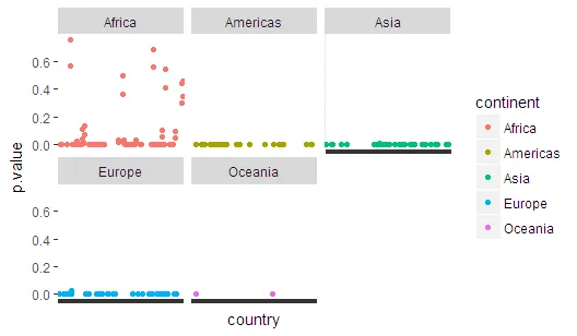
sol2 %>% unnest %>% unnest(tidymodels) %>% 
  ggplot(aes(country,p.value,colour=continent))+geom_point()+
  facet_wrap(~continent)+
  theme(axis.text.x = element_blank())

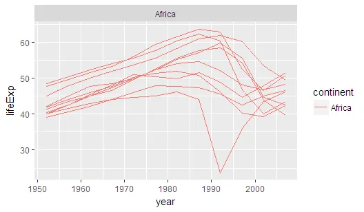
selc <- sol2 %>% unnest %>% unnest(tidymodels) %>% filter(p.value > 0.05) %>% 
  select(country) %>% unique %>% extract2(1)

gapminder %>% filter(country %in% selc ) %>%
  ggplot(aes(year,lifeExp,colour=continent))+geom_line(aes(group=country))+
  facet_wrap(~continent)

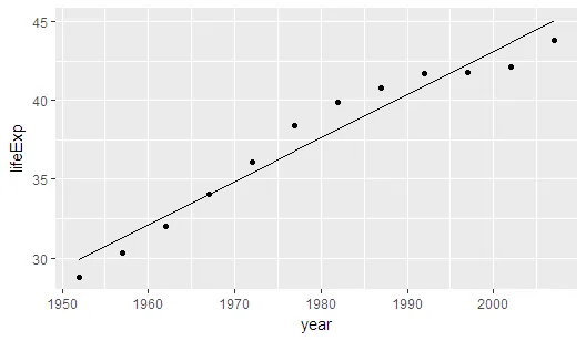
然后，我们可以使用这些模型。

m1 <- sol2 %>% unnest %>% slice(1) %$% models %>% extract2(1)

x <- sol2 %>% unnest %>% slice(1) %>% unnest(by_country) %>% select(year)

pred1 <- data.frame(year = x, lifeExp = predict.lm(m1,x))

sol2 %>% unnest %>% slice(1) %>% unnest(by_country) %>%
  ggplot(aes(year, lifeExp )) + geom_point() +
  geom_line(data=pred1)

在这个例子中，除了学习如何嵌套之外，实际上没有什么好的理由使用这种双重嵌套。但我在工作中找到了一个非常有价值的案例，特别是当您需要一个函数在第三级上运行，在第1级和第2级分组，并将其保存在第2级时 - 当然，我们也可以在第1级上使用for循环，但那又有什么意思呢？;) 我不确定与for循环+ map相比，这个“嵌套”的map表现如何，但我会进行测试。

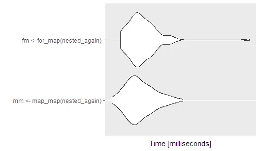
基准测试

看起来它们并没有太大区别

# comparison map_map with for_map
map_map<-function(nested_again){
nested_again %>% mutate(by_continent = map(by_continent, ~.x %>% 
  mutate(models = map(by_country, ~lm(lifeExp ~ year, data = .x) )) )) }

for_map<-function(nested_again){ for(i in 1:length(nested_again[[1]])){
  nested_again$by_continent[[i]] %<>%
  mutate(models = map(by_country, ~lm(lifeExp ~ year, data = .x) )) }}

res<-microbenchmark::microbenchmark(
  mm<-map_map(nested_again), fm<-for_map(nested_again) )

res
# Unit: milliseconds
#                         expr      min       lq     mean   median       uq      max neval cld
#  mm <- map_map(nested_again) 121.0033 144.5530 160.6785 155.2389 174.2915 240.2012   100   a
#  fm <- for_map(nested_again) 131.4312 148.3329 164.7097 157.6589 173.6480 455.7862   100   a

autoplot(res)

- RBA