给定3D点，绘制3D曲面的最简单方法

Question

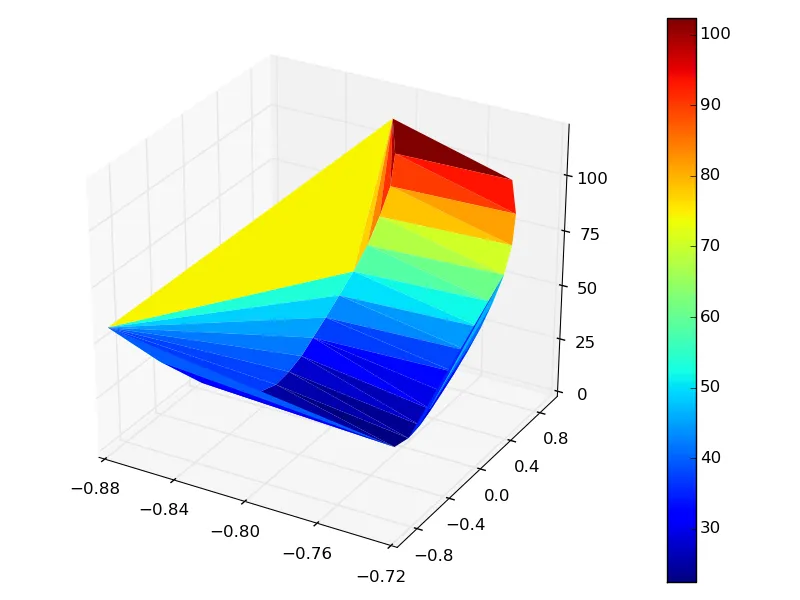
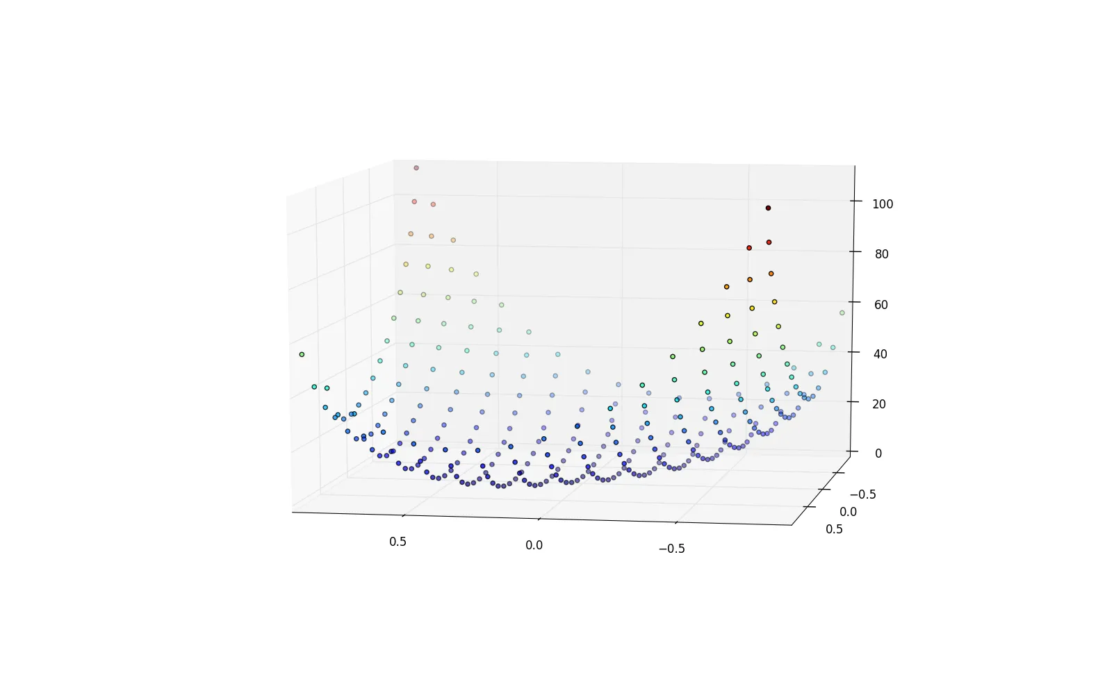
我有很多（289个）带有xyz坐标的3D点，看起来像这样：

在简单绘制三维空间中的点方面，我没问题，但是在绘制曲面方面我遇到了困难。 以下是一些要点：

for i in range(30):
        output.write(str(X[i])+' '+str(Y[i])+' '+str(Z[i])+'\n')

-0.807237702464 0.904373229492 111.428744443
-0.802470821517 0.832159465335 98.572957317
-0.801052795982 0.744231916692 86.485869328
-0.802505546206 0.642324228721 75.279804677
-0.804158144115 0.52882485495 65.112895758
-0.806418040943 0.405733109371 56.1627277595
-0.808515314192 0.275100227689 48.508994388
-0.809879521648 0.139140394575 42.1027499025
-0.810645106092 -7.48279012695e-06 36.8668106345
-0.810676720161 -0.139773175337 32.714580273
-0.811308686707 -0.277276065449 29.5977405865
-0.812331692291 -0.40975978382 27.6210856615
-0.816075037319 -0.535615685086 27.2420699235
-0.823691366944 -0.654350489595 29.1823292975
-0.836688691603 -0.765630198427 34.2275056775
-0.854984518665 -0.86845932028 43.029581434
-0.879261949054 -0.961799684483 55.9594146815
-0.740499820944 0.901631050387 97.0261463995
-0.735011699497 0.82881933383 84.971061395
-0.733021568161 0.740454485354 73.733621269
-0.732821755233 0.638770044767 63.3815970475
-0.733876941678 0.525818698874 54.0655910105
-0.735055978521 0.403303715698 45.90859502
-0.736448900325 0.273425879041 38.935709456
-0.737556181137 0.13826504904 33.096106049
-0.738278724065 -9.73058423274e-06 28.359664343
-0.738507612286 -0.138781586244 24.627237837
-0.738539663773 -0.275090412979 21.857410904
-0.739099040189 -0.406068448513 20.1110519655
-0.741152200369 -0.529726022182 19.7019157715

没有相等的X和Y值。X的取值范围是从-0.8到0.8，Y的取值范围是从-0.9到0.9，Z的取值范围是从0到111。

如果可能的话，如何使用这些点绘制3D曲面图？

- XuMuK

---

这里有另一个例子：https://dev59.com/pWox5IYBdhLWcg3wf0Xl#30539444。此外，请查看这些相关/类似/重复的帖子：https://dev59.com/5XA75IYBdhLWcg3w8-HZ，https://dev59.com/pWox5IYBdhLWcg3wf0Xl，https://dev59.com/i3vaa4cB1Zd3GeqPCWDE，http://stackoverflow.com/q/26074542/3585557，http://stackoverflow.com/q/28389606/3585557，https://dev59.com/zYnda4cB1Zd3GeqPAYnU。 - Steven C. Howell

Answer 1

使用matplotlib的解决方案：

#!/usr/bin/python3

import sys

import matplotlib
import matplotlib.pyplot as plt
from matplotlib.ticker import MaxNLocator
from matplotlib import cm
from mpl_toolkits.mplot3d import Axes3D

import numpy
from numpy.random import randn
from scipy import array, newaxis


# ======
## data:

DATA = array([
    [-0.807237702464, 0.904373229492, 111.428744443],
    [-0.802470821517, 0.832159465335, 98.572957317],
    [-0.801052795982, 0.744231916692, 86.485869328],
    [-0.802505546206, 0.642324228721, 75.279804677],
    [-0.804158144115, 0.52882485495, 65.112895758],
    [-0.806418040943, 0.405733109371, 56.1627277595],
    [-0.808515314192, 0.275100227689, 48.508994388],
    [-0.809879521648, 0.139140394575, 42.1027499025],
    [-0.810645106092, -7.48279012695e-06, 36.8668106345],
    [-0.810676720161, -0.139773175337, 32.714580273],
    [-0.811308686707, -0.277276065449, 29.5977405865],
    [-0.812331692291, -0.40975978382, 27.6210856615],
    [-0.816075037319, -0.535615685086, 27.2420699235],
    [-0.823691366944, -0.654350489595, 29.1823292975],
    [-0.836688691603, -0.765630198427, 34.2275056775],
    [-0.854984518665, -0.86845932028, 43.029581434],
    [-0.879261949054, -0.961799684483, 55.9594146815],
    [-0.740499820944, 0.901631050387, 97.0261463995],
    [-0.735011699497, 0.82881933383, 84.971061395],
    [-0.733021568161, 0.740454485354, 73.733621269],
    [-0.732821755233, 0.638770044767, 63.3815970475],
    [-0.733876941678, 0.525818698874, 54.0655910105],
    [-0.735055978521, 0.403303715698, 45.90859502],
    [-0.736448900325, 0.273425879041, 38.935709456],
    [-0.737556181137, 0.13826504904, 33.096106049],
    [-0.738278724065, -9.73058423274e-06, 28.359664343],
    [-0.738507612286, -0.138781586244, 24.627237837],
    [-0.738539663773, -0.275090412979, 21.857410904],
    [-0.739099040189, -0.406068448513, 20.1110519655],
    [-0.741152200369, -0.529726022182, 19.7019157715],
])

Xs = DATA[:,0]
Ys = DATA[:,1]
Zs = DATA[:,2]


# ======
## plot:

fig = plt.figure()
ax = fig.add_subplot(111, projection='3d')

surf = ax.plot_trisurf(Xs, Ys, Zs, cmap=cm.jet, linewidth=0)
fig.colorbar(surf)

ax.xaxis.set_major_locator(MaxNLocator(5))
ax.yaxis.set_major_locator(MaxNLocator(6))
ax.zaxis.set_major_locator(MaxNLocator(5))

fig.tight_layout()

plt.show() # or:
# fig.savefig('3D.png')

结果：

可能不太美观。但是如果您提供更多的点，它将会变得更漂亮。

- Adobe

Answer 2

请查看Axes3D.plot_surface或其他Axes3D方法。你可以在这里找到示例和灵感，here，here或here。

编辑：

不在规则X-Y网格上的Z数据（一个维度中网格点之间的等距）作为三角形表面进行绘制并不容易。对于给定的不规则（X，Y）坐标集，有多种可能的三角剖分。可以通过“最近邻”Delaunay算法计算一种三角剖分。这可以在matplotlib中完成。但是，它仍然有些繁琐：

http://matplotlib.1069221.n5.nabble.com/Plotting-3D-Irregularly-Triangulated-Surfaces-An-Example-td9652.html

看起来支持将得到改善：

http://matplotlib.org/examples/pylab_examples/tripcolor_demo.html http://matplotlib.1069221.n5.nabble.com/Custom-plot-trisurf-triangulations-tt39003.html

借助http://docs.enthought.com/mayavi/mayavi/auto/example_surface_from_irregular_data.html的帮助，我能够基于mayavi提供一个非常简单的解决方案：

import numpy as np
from mayavi import mlab

X = np.array([0, 1, 0, 1, 0.75])
Y = np.array([0, 0, 1, 1, 0.75])
Z = np.array([1, 1, 1, 1, 2])

# Define the points in 3D space
# including color code based on Z coordinate.
pts = mlab.points3d(X, Y, Z, Z)

# Triangulate based on X, Y with Delaunay 2D algorithm.
# Save resulting triangulation.
mesh = mlab.pipeline.delaunay2d(pts)

# Remove the point representation from the plot
pts.remove()

# Draw a surface based on the triangulation
surf = mlab.pipeline.surface(mesh)

# Simple plot.
mlab.xlabel("x")
mlab.ylabel("y")
mlab.zlabel("z")
mlab.show()

这是一个基于5个点的非常简单的例子。其中4个点位于z级别1：

(0, 0) (0, 1) (1, 0) (1, 1)

其中一个位于z级别2：

(0.75, 0.75)

Delaunay算法可以正确地进行三角剖分，因此表面会按预期绘制出来。

我在Windows上安装了Python(x,y)后，使用以下命令运行了上述代码：

ipython -wthread script.py

- Dr. Jan-Philip Gehrcke

---

Axes34需要用于表面绘图的点，这些点在同一行中。 - XuMuK

构建表面最简单的方法是绘制许多四边形。 - XuMuK