如何使用Matplotlib可视化标量2D数据？

Question

如何使用Matplotlib可视化标量2D数据？

pythonmatplotlib

10

我有一个网格（矩阵 X 和 Y）和标量数据（矩阵 Z），需要对其进行可视化。最好是在点处使用颜色的二维图像，显示该处的 Z 值。

我已经做了一些研究，但没有找到完全符合我的要求的内容。

pyplot.imshow(Z) 看起来很不错，但它不接受我的 X 和 Y 矩阵，所以坐标轴错误，并且无法处理由 X 和 Y 给出的非线性间隔点。

pyplot.pcolor(X,Y,Z) 生成彩色正方形，其颜色对应于其中一个角落的数据，因此它会误导数据（应该在中心或其他位置显示数据）。此外，它会忽略数据矩阵的两个边缘。

我确信在 Matplotlib 中肯定存在某种更好的方法，但文档使得很难获得概述。因此，我想问是否有其他人知道更好的方法。如果可以刷新矩阵 Z 来制作动画，则奖励更好。

- Eskil

4个回答

2

如果您的网格具有统一的间距，您可以继续使用pcolor，但只需为了将数据居中于特定值而不是角落而移动X和Y。您还可以使用散点图在确切的X和Y点上明确放置某些大小的点，然后将颜色设置为Z：

x = numpy.arange(10)
y = numpy.arange(10)
X,Y = numpy.meshgrid(x,y)
Z = numpy.arange(100).reshape((10,10))
scatter(X,Y,c=Z,marker='s',s=1500) 
#I picked a marker size that basically overlapped the symbols at the edges
axis('equal')

或者：

pcolor(X+0.5,Y+0.5,Z)
axis('equal')

或者像Paul建议的那样，使用其中一个轮廓函数。

- JoshAdel

1

如果有人在阅读这篇文章时正在寻找我所需要的内容，我已经采用了上述示例并进行了修改，使用imshow来显示一组帧的输入堆栈，而不是即时生成和使用轮廓。从一个形状为(nBins, nBins, nBins)的图像的3D数组开始，称为frames。

def animate_frames(frames):
    nBins   = frames.shape[0]
    frame   = frames[0]
    tempCS1 = plt.imshow(frame, cmap=plt.cm.gray)
    for k in range(nBins):
        frame   = frames[k]
        tempCS1 = plt.imshow(frame, cmap=plt.cm.gray)
        del tempCS1
        fig.canvas.draw()
        #time.sleep(1e-2) #unnecessary, but useful
        fig.clf()

fig = plt.figure()
ax  = fig.add_subplot(111)

win = fig.canvas.manager.window
fig.canvas.manager.window.after(100, animate_frames, frames)

我也发现了一个更简单的方法来完成整个过程，虽然不太健壮：

fig = plt.figure()

for k in range(nBins):
    plt.clf()
    plt.imshow(frames[k],cmap=plt.cm.gray)
    fig.canvas.draw()
    time.sleep(1e-6) #unnecessary, but useful

请注意，这两个似乎只能与ipython --pylab=tk一起使用，也就是说backend = TkAgg

感谢您对所有事情的帮助。

- CavemanPhD

0

以下函数在边界处创建大小为一半的方框（如附图所示）。

import matplotlib.pyplot as plt
import numpy as np
from scipy.ndimage.filters import convolve

def pcolor_all(X, Y, C, **kwargs):
    X = np.concatenate([X[0:1,:], X], axis=0)
    X = np.concatenate([X[:,0:1], X], axis=1)

    Y = np.concatenate([Y[0:1,:], Y], axis=0)
    Y = np.concatenate([Y[:,0:1], Y], axis=1)

    X = convolve(X, [[1,1],[1,1]])/4
    Y = convolve(Y, [[1,1],[1,1]])/4

    plt.pcolor(X, Y, C, **kwargs)

X, Y = np.meshgrid(
    [-1,-0.5,0,0.5,1],
    [-2,-1,0,1,2])

C = X**2-Y**2

plt.figure(figsize=(4,4))

pcolor_all(X, Y, C, cmap='gray')

plt.savefig('plot.png')

- klaus se

网页内容由stack overflow 提供, 点击上面的

可以查看英文原文，
原文链接

- Paul · Accepted Answer

这看起来很不错，但效率低下：

from pylab import *
origin = 'lower'

delta = 0.025

x = y = arange(-3.0, 3.01, delta)
X, Y = meshgrid(x, y)
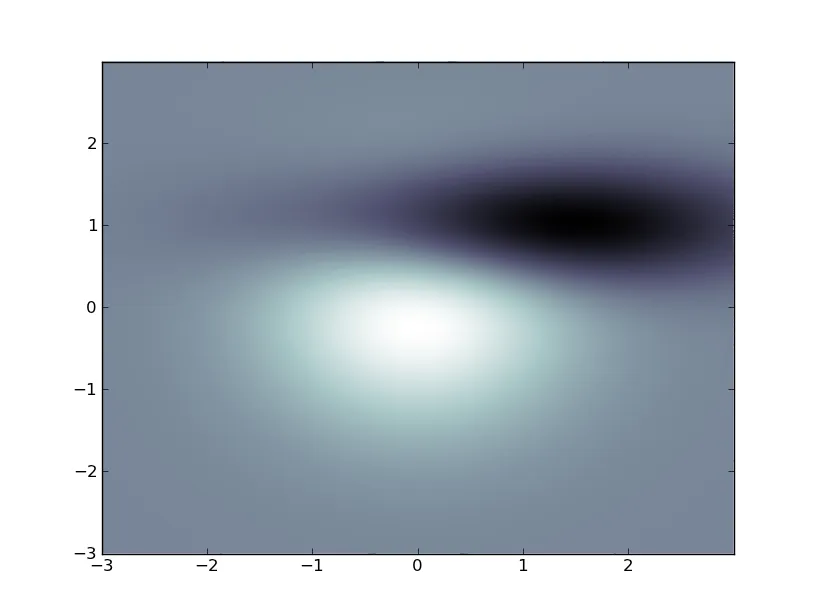
Z1 = bivariate_normal(X, Y, 1.0, 1.0, 0.0, 0.0)
Z2 = bivariate_normal(X, Y, 1.5, 0.5, 1, 1)
Z = 10 * (Z1 - Z2)

nr, nc = Z.shape

CS = contourf(
    X, Y, Z,
    levels = linspace(Z.min(), Z.max(), len(x)),
    ls = '-',
    cmap=cm.bone,
    origin=origin)

CS1 = contour(
    CS,
    levels = linspace(Z.min(), Z.max(), len(x)),
    ls = '-',
    cmap=cm.bone,
    origin=origin)

show()

如果是我，我会使用scipy.interpolate重新插值数据到一个规则的网格上，并使用imshow()，设置extents以固定坐标轴。

fine contour

编辑（根据评论）：

像这样可以实现轮廓图的动画，但是，如我所说，上述方法是轮廓图函数的滥用，非常低效。实现你想要的最有效的方法是使用SciPy。你安装了吗？

import matplotlib
matplotlib.use('TkAgg') # do this before importing pylab
import time
import matplotlib.pyplot as plt

fig = plt.figure()
ax = fig.add_subplot(111)

def animate():
    origin = 'lower'
    delta = 0.025

    x = y = arange(-3.0, 3.01, delta)
    X, Y = meshgrid(x, y)
    Z1 = bivariate_normal(X, Y, 1.0, 1.0, 0.0, 0.0)
    Z2 = bivariate_normal(X, Y, 1.5, 0.5, 1, 1)
    Z = 10 * (Z1 - Z2)

    CS1 = ax.contourf(
        X, Y, Z,
        levels = linspace(Z.min(), Z.max(), 10),
        cmap=cm.bone,
        origin=origin)

    for i in range(10):
        tempCS1 = contourf(
            X, Y, Z,
            levels = linspace(Z.min(), Z.max(), 10),
            cmap=cm.bone,
            origin=origin)
        del tempCS1
        fig.canvas.draw()
        time.sleep(0.1)
        Z += x/10

win = fig.canvas.manager.window
fig.canvas.manager.window.after(100, animate)
plt.show()