预测群体的新值

Question

我已经为数据框中的每个组计算了不同的回归：

DF.L <- DF %>%
group_by(Channel) %>%
do(Fit = rlm(L ~ -1 + Y + I(Y^2), data = .))

我想将这组回归应用于另一个数据框。为此，我正在测试如何将其应用于相同的数据框：

DF %>%
group_by(Channel) %>%
do({
    Lfit <- predict(subset(DF.L, Channel == unique(.$Channel))$Fit, .)
    data.frame(., Lfit)
})
glimpse(DF)

但我不断地收到这个错误信息：

Error in UseMethod("predict") : 
  no applicable method for 'predict' applied to an object of class "list"
Calls: %>% ... do_.grouped_df -> eval -> eval -> predict -> predict

我到底做错了什么？

- Medical physicist

Answer 1

使用内置的ChickWeight数据：

library(dplyr)
library(MASS)
library(broom)
library(tidyr)
library(ggplot2)


head(ChickWeight)

  weight Time Chick Diet
1     42    0     1    1
2     51    2     1    1
3     59    4     1    1
4     64    6     1    1
5     76    8     1    1
6     93   10     1    1

适配一些模型

ChickWeight_models <- ChickWeight %>% 
  group_by(Diet) %>% 
  do(fit = MASS::rlm(weight ~ Time + I(Time^2), data = .))

ChickWeight_models

Source: local data frame [4 x 2]
Groups: <by row>

# A tibble: 4 x 2
    Diet       fit
* <fctr>    <list>
1      1 <S3: rlm>
2      2 <S3: rlm>
3      3 <S3: rlm>
4      4 <S3: rlm>

我创建了一个与你的DF.L非常相似的对象。它是一个框架，有四个组，每个组都有一个名为fit的列表列中的rlm对象。

---

准备一些测试数据

现在我要准备一些数据来测试这个模型。在这种情况下，我将只取原始数据并对每个变量添加一些噪声。

ChickWeight_simulated <- ChickWeight %>% 
  mutate(Time = Time + runif(length(Time)),
         weight = weight + rnorm(length(weight)))

ChickWeight_simulated 

    weight       Time Chick Diet
1 42.72075  0.9786272     1    1
2 51.12669  2.8399631     1    1
3 58.64632  4.4576380     1    1
4 63.77617  6.1083591     1    1
5 75.40434  8.1051792     1    1
6 91.75830 10.7899030     1    1

现在我们想把模型的数据框与新的测试数据结合起来。首先，我们使用group_by和tidyr::nest对模拟数据进行分组。这将创建一个包含四个组和一个名为data的列表列的数据框对象，其中每个元素都包含一个汇总的数据框。

ChickWeight_simulated %>% group_by(Diet) %>% nest()

# A tibble: 4 x 2
    Diet               data
  <fctr>             <list>
1      1 <tibble [220 x 3]>
2      2 <tibble [120 x 3]>
3      3 <tibble [120 x 3]>
4      4 <tibble [118 x 3]>

---

将原始模型添加到新数据中

然后，我们可以将其与模型数据框连接：

ChickWeight_simulated %>% group_by(Diet) %>% nest() %>% 
  full_join(ChickWeight_models)

# A tibble: 4 x 3
    Diet               data       fit
  <fctr>             <list>    <list>
1      1 <tibble [220 x 3]> <S3: rlm>
2      2 <tibble [120 x 3]> <S3: rlm>
3      3 <tibble [120 x 3]> <S3: rlm>
4      4 <tibble [118 x 3]> <S3: rlm>

现在我们再次按Diet分组，并使用broom :: augment在新的模拟数据上对每个模型进行预测。由于每个组只有一行，因此每个列表列都有一个元素，我们必须将该单个元素从每个列表列中提取出来，以便使用[[1]]进行使用。

ChickWeight_simulated_predicted <-
ChickWeight_simulated %>% group_by(Diet) %>% nest() %>% 
  full_join(ChickWeight_models) %>% 
  group_by(Diet) %>% 
  do(augment(.$fit[[1]], newdata = .$data[[1]])) 

head(ChickWeight_simulated_predicted)

# A tibble: 6 x 6
# Groups:   Diet [1]
    Diet   weight       Time Chick  .fitted  .se.fit
  <fctr>    <dbl>      <dbl> <ord>    <dbl>    <dbl>
1      1 42.72075  0.9786272     1 43.62963 2.368838
2      1 51.12669  2.8399631     1 51.80855 1.758385
3      1 58.64632  4.4576380     1 59.67606 1.534051
4      1 63.77617  6.1083591     1 68.43218 1.534152
5      1 75.40434  8.1051792     1 80.00678 1.647612
6      1 91.75830 10.7899030     1 97.26450 1.726331

---

健全性检查

为了证明这个模型真正只使用了特定级别饮食的模拟数据，我们可以可视化模型拟合。

ChickWeight_simulated_predicted %>% 
  ggplot(aes(Time, weight)) + 
  geom_point(shape = 1) + 
  geom_ribbon(aes(Time, 
                  ymin = .fitted-1.96*.se.fit, 
                  ymax = .fitted+1.96*.se.fit),
              alpha = 0.5, fill = "black") +
  geom_line(aes(Time, .fitted), size = 1, color = "red") +
  facet_wrap(~Diet)

- Brian

---

太好了！但在我看来，tidyverse 应该让 @hadley 更容易些。 - Medical physicist

Answer 2

我认为您的错误来自于如何调用predict。我无法修复您的确切代码，但这里有一种简单的方法可以从您的模型中获取预测结果。使用purrr和nest的更复杂方法在此处进行了概述：http://ijlyttle.github.io/isugg_purrr/presentation.html#(1) 更新-使用purrr和nest的方法

只需添加这个以展示在tidyverse中可以很容易地完成，使用predict即可。有关更多详细信息，请参见上面的链接。

library(tidyverse)

# shuffle the rows to mix up the species
set.seed(1234)
myiris <- iris[sample(nrow(iris), replace = F),]

# create first dataset - use the first 50 rows for running the model
iris_nested <- 
    myiris[1:50,] %>% 
    nest(-Species) %>% 
    rename(myorigdata = data)

# create second dataset - use the other 100 rows for making predictions
new_iris_nested <- 
    myiris[51:150,] %>% 
    nest(-Species) %>% 
    rename(mynewdata = data)

# make a model function
my_rlm <- function(df) {
    MASS::rlm(Sepal.Length ~ Petal.Length + Petal.Width, data = df)
}

# get the predictions (see the GitHub link above which breaks this into steps)
predictions_tall <- 
    iris_nested %>% 
    mutate(my_model = map(myorigdata, my_rlm)) %>% 
    full_join(new_iris_nested, by = "Species") %>% 
    mutate(my_new_pred = map2(my_model, mynewdata, predict)) %>% 
    select(Species, mynewdata, my_new_pred) %>% 
    unnest(mynewdata, my_new_pred) %>% 
    rename(modeled = my_new_pred, measured = Sepal.Length) %>%
    gather("Type", "Sepal.Length", modeled, measured)

嵌套的predictions_tall对象看起来像这样：

predictions_tall %>% nest(-Species, -type) %>% as.tibble()
# A tibble: 6 x 3
     Species     type                  data
      <fctr>    <chr>                <list>
1     setosa  modeled <data.frame [32 x 4]>
2 versicolor  modeled <data.frame [33 x 4]>
3  virginica  modeled <data.frame [35 x 4]>
4     setosa measured <data.frame [32 x 4]>
5 versicolor measured <data.frame [33 x 4]>
6  virginica measured <data.frame [35 x 4]>

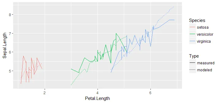
最后，展示预测结果的图表：

predictions_tall %>%
    ggplot(aes(x = Petal.Length, y = Sepal.Length)) +
    geom_line(aes(color = Species, linetype = Type))

翻译 - the broom way

我现在已经更新，只使用每个组的模型计算预测。

这种方法使用broom包-具体来说是augment函数-添加拟合值。更多信息请参见此处：https://cran.r-project.org/web/packages/broom/vignettes/broom.html

由于您没有提供数据，在这里我使用iris。

library(tidyverse)
library(broom)

# first shuffle around the rows of iris
set.seed(1234)
myiris <- iris[sample(nrow(iris), replace = F),]

# first data - first 25 rows for running the models on
origiris <- 
    myiris[1:25,] %>% 
    nest(-Species) %>% 
    rename(origdata = data)

# second data - last 50 rows for predicting on
prediris <- 
    myiris[101:150,] %>% 
    nest(-Species) %>% 
    rename(preddata = data)


# estimate models on the first 25 rows
# a separate model is estimated for each species
iris_mod <- 
    origiris %>% 
    mutate(mod = map(origdata, ~ MASS::rlm(Sepal.Length ~ Petal.Length + Petal.Width, data = .)))

首先为原始数据集获取拟合值（非必需，仅供说明）：

# get fitted values for the first dataset (origdata)
origiris_aug <-  
    iris_mod %>% 
    mutate(origpred = map(mod, augment)) %>% 
    unnest(origpred) %>% 
    as.tibble()

原始的iris_aug预测数据框如下所示：

origiris_aug
# A tibble: 25 x 10
   Species .rownames Sepal.Length Petal.Length Petal.Width  .fitted   .se.fit      .resid
    <fctr>     <chr>        <dbl>        <dbl>       <dbl>    <dbl>     <dbl>       <dbl>
 1  setosa        18          5.1          1.4         0.3 5.002797 0.1514850  0.09720290
 2  setosa         2          4.9          1.4         0.2 4.931824 0.1166911 -0.03182417
 3  setosa        34          5.5          1.4         0.2 4.931824 0.1166911  0.56817583
 4  setosa        40          5.1          1.5         0.2 4.981975 0.1095883  0.11802526
 5  setosa        39          4.4          1.3         0.2 4.881674 0.1422123 -0.48167359
 6  setosa        36          5.0          1.2         0.2 4.831523 0.1784156  0.16847698
 7  setosa        25          4.8          1.9         0.2 5.182577 0.2357614 -0.38257703
 8  setosa        31          4.8          1.6         0.2 5.032125 0.1241074 -0.23212531
 9  setosa        42          4.5          1.3         0.3 4.952647 0.1760223 -0.45264653
10  setosa        21          5.4          1.7         0.2 5.082276 0.1542594  0.31772411
# ... with 15 more rows, and 2 more variables: .hat <dbl>, .sigma <dbl>

现在您实际想要的是对新数据集进行预测：

# get fitted values for the second dataset (preddata)
# each model is fitted to the appropriate species' nested dataframe

prediris_aug <- 
    iris_mod %>% 
    inner_join(prediris, by = "Species") %>% 
    map2_df(.x = iris_mod$mod, .y = prediris$preddata, .f = ~augment(.x, newdata = .y)) %>% 
    as.tibble()

prediris_aug 数据框如下所示：

prediris_aug
# A tibble: 50 x 7
   .rownames Sepal.Length Sepal.Width Petal.Length Petal.Width  .fitted  .se.fit
       <chr>        <dbl>       <dbl>        <dbl>       <dbl>    <dbl>    <dbl>
 1       105          6.5         3.0          5.8         2.2 8.557908 3.570269
 2       115          5.8         2.8          5.1         2.4 8.348800 3.666631
 3       117          6.5         3.0          5.5         1.8 8.123565 3.005888
 4       139          6.0         3.0          4.8         1.8 7.772511 2.812748
 5       103          7.1         3.0          5.9         2.1 8.537086 3.475224
 6       107          4.9         2.5          4.5         1.7 7.551086 2.611123
 7       119          7.7         2.6          6.9         2.3 9.180537 4.000412
 8       135          6.1         2.6          5.6         1.4 7.889823 2.611457
 9       124          6.3         2.7          4.9         1.8 7.822661 2.838502
10       118          7.7         3.8          6.7         2.2 9.009263 3.825613
# ... with 40 more rows

- meenaparam

---

不错的@meenaparam，但是每行只应该有一个预测，根据该行的物种值。 - Medical physicist

@Medicalphysicist 在 do 前使用 group_by 意味着我们为每个物种水平拟合一个模型，因此我们最终会有三个模型进行预测。在您的数据中，您是否只想基于相同分组值构建的模型对新观测结果进行预测？ - meenaparam

是的。在我的情况下，使用来自另一个频道的模型没有意义。 - Medical physicist

@Medicalphysicist 没问题，我没有意识到这一点。你现在有一个答案了，但是我现在会更新这个答案，展示一下使用purrr的方式，我觉得这样做会更容易一些。 - meenaparam

谢谢！这是一个非常有趣的选项。 - Medical physicist