我正在寻找有效的方法来去除我的数据中的异常值。我尝试了一些在StackOverflow和其他地方找到的解决方案,但是它们都对我没有起作用(在1993年6月、1994年8月和1995年3月的样本数据中,应该检测到并删除4个高值,分别为21637、19590、21659和200000)。非常感谢任何建议!
以下是我目前测试过的内容:
数据概述如何从数据集中删除异常值
类似于第一种方法的问题
以下是我目前测试过的内容:
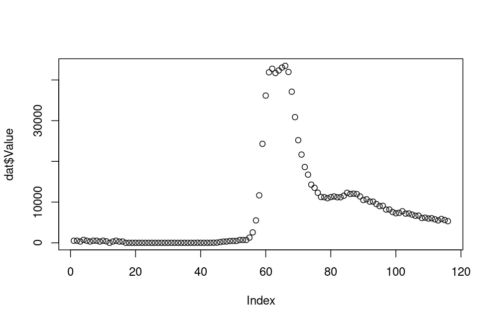
数据概述

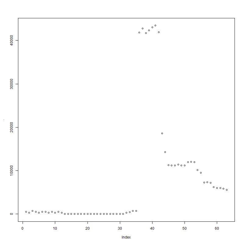
仍然存在3个异常值,并且在时间序列的末尾删除了许多合法的高值。
y <- dat$Value
y_filter <- y[!y %in% boxplot.stats(y)$out]
plot(y_filter)

类似于第一种方法的问题
FindOutliers <- function(data) {
  data <- data[!is.na(data)]
  lowerq = quantile(data)[2]
  upperq = quantile(data)[4]
  iqr = upperq - lowerq #Or use IQR(data)
  # we identify extreme outliers
  extreme.threshold.upper = (iqr * 1.5) + upperq
  extreme.threshold.lower = lowerq - (iqr * 1.5)
  result <- which(data > extreme.threshold.upper | data < extreme.threshold.lower)

  return(result)
}

# use the function to identify outliers
temp <- FindOutliers(y)
# remove the outliers
y1 <- y[-temp]
# show the data with the outliers removed
y1
#>   [1]   511   524   310   721   514   318   511   511   318   510 21637     0
#>  [13]   319   511   305   317     0     0     0     0     0     0     0     0
#>  [25] 19590     0     0     0     0     0     0     0     0 21659     0     0
#>  [37]     0     0    19     7     0     5     9    21    50   187   291   321
#>  [49]   445   462   462   695   694   693  1276  2560  5500 11663 24307 25205
#>  [61] 21667 18610 16739 14294 13517 12296 11247 11209 10954 11228 11387 11190
#>  [73] 11193 11562 12279 11994 12073 11965 11386 10512 10677 10115 10118  9530
#>  [85]  9016  9086  8167  8171  7561  7268  7359  7753  7168  7206  6926  6646
#>  [97]  6674  6100  6177  5975  6033  5767  5497  5862  5594  5319
plot(y1)

library(performance)
outliers_list <- check_outliers(y) # Find outliers
outliers_list # Show the row index of the outliers
#> 9 outliers detected: cases 60, 61, 62, 63, 64, 65, 66, 67, 68.
#> - Based on the following method and threshold: zscore_robust (3.291).
#> - For variable: y.
#>
#> -----------------------------------------------------------------------------
#> Outliers per variable (zscore_robust):
#>
#> $y
#>    Row Distance_Zscore_robust
#> 60  60               3.688817
#> 61  61               4.384524
#> 62  62               4.491276
#> 63  63               4.362517
#> 64  64               4.438994
#> 65  65               4.525319
#> 66  66               4.576871
#> 67  67               4.393886
#> 68  68               3.804809
str(outliers_list)
#>  'check_outliers' logi [1:116] FALSE FALSE FALSE FALSE FALSE FALSE ...
#>  - attr(*, "data")='data.frame': 116 obs. of  4 variables:
#>   ..$ Row                   : int [1:116] 1 2 3 4 5 6 7 8 9 10 ...
#>   ..$ Distance_Zscore_robust: num [1:116] 0.645 0.643 0.669 0.619 0.644 ...
#>   ..$ Outlier_Zscore_robust : num [1:116] 0 0 0 0 0 0 0 0 0 0 ...
#>   ..$ Outlier               : num [1:116] 0 0 0 0 0 0 0 0 0 0 ...
#>  - attr(*, "threshold")=List of 1
#>   ..$ zscore_robust: num 3.29
#>  - attr(*, "method")= chr "zscore_robust"
#>  - attr(*, "text_size")= num 3
#>  - attr(*, "variables")= chr "y"
#>  - attr(*, "raw_data")='data.frame': 116 obs. of  1 variable:
#>   ..$ y: num [1:116] 511 524 310 721 514 318 511 511 318 510 ...
#>  - attr(*, "outlier_var")=List of 1
#>   ..$ zscore_robust:List of 1
#>   .. ..$ y:'data.frame': 9 obs. of  2 variables:
#>   .. .. ..$ Row                   : int [1:9] 60 61 62 63 64 65 66 67 68
#>   .. .. ..$ Distance_Zscore_robust: num [1:9] 3.69 4.38 4.49 4.36 4.44 ...
#>  - attr(*, "outlier_count")=List of 2
#>   ..$ zscore_robust:'data.frame':    0 obs. of  2 variables:
#>   .. ..$ Row            : int(0)
#>   .. ..$ n_Zscore_robust: int(0)
#>   ..$ all          :'data.frame':    0 obs. of  2 variables:
#>   .. ..$ Row            : num(0)
#>   .. ..$ n_Zscore_robust: num(0)

y[!outliers_list]
#>   [1]   511   524   310   721   514   318   511   511   318   510 21637     0
#>  [13]   319   511   305   317     0     0     0     0     0     0     0     0
#>  [25] 19590     0     0     0     0     0     0     0     0 21659     0     0
#>  [37]     0     0    19     7     0     5     9    21    50   187   291   321
#>  [49]   445   462   462   695   694   693  1276  2560  5500 11663 24307 30864
#>  [61] 25205 21667 18610 16739 14294 13517 12296 11247 11209 10954 11228 11387
#>  [73] 11190 11193 11562 12279 11994 12073 11965 11386 10512 10677 10115 10118
#>  [85]  9530  9016  9086  8167  8171  7561  7268  7359  7753  7168  7206  6926
#>  [97]  6646  6674  6100  6177  5975  6033  5767  5497  5862  5594  5319

par(mfrow = c(2,1), oma = c(2,2,0,0) + 0.1, mar = c(0,0,2,1) + 0.2)
plot(y)
plot(y[!outliers_list])

测试数据
library(tibble)

dat <- tibble::tribble(
  ~DateTime, ~Value,
  "1993-06-06 11:00:00",     NA,
  "1993-06-06 12:00:00",    524,
  "1993-06-06 13:00:00",    310,
  "1993-06-06 14:00:00",    721,
  "1993-06-06 15:00:00",    514,
  "1993-06-06 16:00:00",    318,
  "1993-06-06 17:00:00",    511,
  "1993-06-06 18:00:00",    511,
  "1993-06-06 19:00:00",    318,
  "1993-06-06 20:00:00",    510,
  "1993-06-06 21:00:00",  21637,
  "1993-06-06 22:00:00",     NA,
  "1993-06-06 23:00:00",    319,
  "1993-06-07 24:00:00",    511,
  "1993-06-07 01:00:00",    305,
  "1993-06-07 02:00:00",    317,
  "1994-08-25 06:00:00",      0,
  "1994-08-25 07:00:00",      0,
  "1994-08-25 08:00:00",      0,
  "1994-08-25 09:00:00",     NA,
  "1994-08-25 10:00:00",      0,
  "1994-08-25 11:00:00",      0,
  "1994-08-25 12:00:00",      0,
  "1994-08-25 13:00:00",      0,
  "1994-08-25 14:00:00",  19590,
  "1994-08-26 06:00:00",      0,
  "1994-08-26 07:00:00",      0,
  "1994-08-26 08:00:00",      0,
  "1994-08-26 09:00:00",      0,
  "1994-08-26 10:00:00",     NA,
  "1994-08-26 11:00:00",     NA,
  "1994-08-26 12:00:00",      0,
  "1994-08-26 13:00:00",      0,
  "1994-08-26 14:00:00",  21659,
  "1994-08-26 15:00:00",      0,
  "1994-08-26 16:00:00",      0,
  "1994-08-26 17:00:00",      0,
  "1994-08-26 20:00:00",      0,
  "1994-08-26 21:00:00",     19,
  "1994-08-26 22:00:00",     NA,
  "1995-03-09 18:00:00",     NA,
  "1995-03-09 19:00:00",     NA,
  "1995-03-09 20:00:00",      9,
  "1995-03-09 21:00:00",     21,
  "1995-03-09 22:00:00",     50,
  "1995-03-09 23:00:00",    187,
  "1995-03-10 24:00:00",    291,
  "1995-03-10 01:00:00",    321,
  "1995-03-10 02:00:00",    445,
  "1995-03-10 03:00:00",  2e+05,
  "1995-03-10 04:00:00",    462,
  "1995-03-10 05:00:00",    695,
  "1995-03-10 06:00:00",    694,
  "1995-03-10 07:00:00",    693,
  "1995-03-10 08:00:00",   1276,
  "1995-03-10 09:00:00",   2560,
  "1995-03-10 10:00:00",   5500,
  "1995-03-10 11:00:00",  11663,
  "1995-03-10 12:00:00",  24307,
  "1995-03-10 15:00:00",  36154,
  "1995-03-10 17:00:00",  41876,
  "1995-03-10 18:00:00",  42754,
  "1995-03-10 19:00:00",     NA,
  "1995-03-10 20:00:00",     NA,
  "1995-03-10 21:00:00",  43034,
  "1995-03-10 22:00:00",  43458,
  "1995-03-10 23:00:00",  41953,
  "1995-03-11 24:00:00",  37108,
  "1995-03-11 01:00:00",  30864,
  "1995-03-11 02:00:00",  25205,
  "1995-03-11 03:00:00",     NA,
  "1995-03-11 04:00:00",     NA,
  "1995-03-11 05:00:00",     NA,
  "1995-03-11 06:00:00",     NA,
  "1995-03-11 07:00:00",  13517,
  "1995-03-11 08:00:00",  12296,
  "1995-03-11 09:00:00",  11247,
  "1995-03-11 10:00:00",  11209,
  "1995-03-11 11:00:00",  10954,
  "1995-03-11 12:00:00",  11228,
  "1995-03-11 13:00:00",  11387,
  "1995-03-11 14:00:00",  11190,
  "1995-03-11 15:00:00",  11193,
  "1995-03-11 16:00:00",  11562,
  "1995-03-11 17:00:00",  12279,
  "1995-03-11 18:00:00",  11994,
  "1995-03-11 19:00:00",  12073,
  "1995-03-11 20:00:00",  11965,
  "1995-03-11 21:00:00",  11386,
  "1995-03-11 22:00:00",  10512,
  "1995-03-11 23:00:00",  10677,
  "1995-03-12 24:00:00",  10115,
  "1995-03-12 01:00:00",  10118,
  "1995-03-12 02:00:00",   9530,
  "1995-03-12 03:00:00",   9016,
  "1995-03-12 04:00:00",   9086,
  "1995-03-12 05:00:00",   8167,
  "1995-03-12 06:00:00",   8171,
  "1995-03-12 07:00:00",   7561,
  "1995-03-12 08:00:00",   7268,
  "1995-03-12 09:00:00",   7359,
  "1995-03-12 10:00:00",   7753,
  "1995-03-12 11:00:00",   7168,
  "1995-03-12 12:00:00",   7206,
  "1995-03-12 13:00:00",   6926,
  "1995-03-12 14:00:00",   6646,
  "1995-03-12 15:00:00",   6674,
  "1995-03-12 16:00:00",   6100,
  "1995-03-12 17:00:00",   6177,
  "1995-03-12 18:00:00",   5975,
  "1995-03-12 19:00:00",   6033,
  "1995-03-12 20:00:00",   5767,
  "1995-03-12 21:00:00",   5497,
  "1995-03-12 22:00:00",   5862,
  "1995-03-12 23:00:00",   5594,
  "1995-03-13 24:00:00",     NA
)
2023-10-05创建,使用reprex v2.0.2


sp <- smooth.spline(dat$Value); dev <- abs(dat$Value - sp$y); dat$Value[dev > quantile(dev, 0.975)]看起来给出了一些有意义的结果? - undefined